This tutorial was created by Dani Cosme and Sam Chavez as part of PSY 607: Data Science Seminar at the University of Oregon.
The tutorial and associated files can also be found on GitHub.
Overview of the tutorial
- Background
- Learn the basics
- Explore advanced features
- Check out the
hugo-academictheme - Publish your website to GitHub
Background
Most of the information in this tutorial is taken from a few amazing resources on using the blogdown package to create static websites in RStudio using R Markdown:
- blogdown: Creating Websites with R Markdown
- Various presentations and posts by Alison Hill
Why use RStudio to make static websites?
- It’s easy
- It’s free
- It’s a simple way to share your code and analyses
What is blogdown?
blogdown is a package that leverages R Markdown and Hugo to create static websites.
What is Hugo?
Hugo is a static website generator. Static websites are collections of HTML files and the external dependencies referenced within them. More on Hugo here.
Learn the basics
Install blogdown and hugo
if (!require(blogdown)) {
  install.packages("blogdown")
}
blogdown::install_hugo()
Update hugo if necessary
blogdown::hugo_version()
blogdown::update_hugo()
Create a website using the default lithium template
There are a number of ways to create a new website project. You can create it using the IDE by clicking File > New Project > New Directory > Website Using Blogdown or by simply specifying the path to the new website as a argument in the blogdown::new_site() function. Make sure that you specify the new directory (e.g. the name of the folder you would like to create) in the path.
Here we’ll create the website one level above our current working directory. The reason for doing this is that our current working directory is a git repository and if we try to publish this later, it will cause problems (it’s not straight forward to have a repo inside of a repo).
blogdown::new_site("../default-site")You can also specify a theme when creating your new site. The default is the lithium theme, but there are a variety of other Hugo themes available. We’ll use the hugo-academic theme later in the tutorial.
blogdown::new_site(theme = 'yihui/hugo-lithium')
blogdown::new_site(theme = 'devcows/hugo-universal-theme')
blogdown::new_site(theme = 'gcushen/hugo-academic')
Render the site
Anytime you want to render the site, you can do so by either clicking Addins > Serve Site or executing the blogdown::serve_site() function. This function should be executed from the site directory, so if you are not currently in that directory, make sure to change you current working directory to the site directory.
setwd("../default-site/")
blogdown::serve_site()
Where does the content live?
Take a look at what’s in the site directory.
Key components:
* config.toml = configuration file that the user edits to customize their site
* /content/ = where the actual content (e.g. pages, posts live)
* /public/ = the directory containing the website for online deployment
* /layouts/ = where you’ll place code to override the original template design
* /static/ = where content such as images and CSS code are stored
* /theme/ = where the theme template is stored
config.toml file
The configuration file is where global variables and settings are defined. More about configuration files and the variables specified within it here. More information on TOML syntax here.
Edit config.toml
Change the site name
title = "Dani Cosme, M.S."Enable emojis
enableEmoji = trueHomepage
Create a file called index.html in the layouts/ directory.
touch ../default-site/layouts/index.htmlCopy the following text into layouts/index.html. I borrowed this code from Alison Hill’s awesome blogdown tutorial, but you could write your own html code to create the layout for your homepage.
{{ partial "header" . }}

<div class="intro">
        <div><center><img class="center-image" src={{ .Site.Params.img }} width="20%"/></center></div>

        <h1><center>{{ markdownify .Title }}</center></h1>

        <h2><center>{{ markdownify .Site.Params.Description }}</center></h2>

</div>


{{ partial "footer" . }}
We referenced a field.Site.Params.img, but it currently doesn’t exist. Let’s add it to config.toml and also update the site description.
[params]
    description = "Welcome to my website!<br>Here is a bunch of text about me.<br>Yada yada yada."
    img = "https://avatars1.githubusercontent.com/u/11858670?s=460&v=4"
Since the posts are no longer on linked from the landing page, let’s add the Posts page to the navigation bar by adding it as a field in config.toml:
[[menu.main]]
    name = "Posts"
    url = "/post/"
About page
Open /content/about.md and check it out. Add the following text to the about.md file and look at the difference.
Because we enabled emojis in `config.toml`, we can use them here. I ❤️ emojis!

Posts are written in plain markdown. Here is some useful syntax. More on plain markdown in the default post [A Plain Markdown Post](../2016/12/30/a-plain-markdown-post/). There's also lots more information in the digital book [*blogdown: Creating Websites with R Markdown*](https://bookdown.org/yihui/blogdown/output-format.html).

## h2 header
### h3 header
#### h4 header

**bold**<br>
*italics*<br>
~~strikethrough~~

Also check out [Cory's awesome markdown tutorial](https://github.com/uodatascience/markdown) for more markdown magic.

Note: you can write in html.

<h4> Embed a gif <br>
<img src="https://media.giphy.com/media/l0Nwvo3slpo6nS0PC/giphy.gif" alt="neato">

<h4> Embed a calendar <br>
<iframe src="https://calendar.google.com/calendar/embed?src=beo4lsbjns0kqovh8nktjou8l4%40group.calendar.google.com&ctz=America%2FLos_Angeles" style="border: 0" width="800" height="600" frameborder="0" scrolling="no"></iframe>
Pages
Create a new page called CV in the content folder.
setwd("../default-site/")
blogdown::new_content("content/cv")
Copy the following text into the document:
---
title: ''
date: '2018-06-03 23:25:08 GMT'
---

<div style="text-align: right"><h1>DANI COSME</div>
<div style="text-align: right">dcosme@uoregon.edu</div>
<div style="text-align: right"><a href="http://dcosme.github.io">dcosme.github.io</a></div>

### EDUCATION //
**Doctoral Candidate, Psychology, 2015-present**<br>
University of Oregon (Eugene, OR)<br>
Advisors: Drs. Jennifer Pfeifer & Elliot Berkman

### PUBLICATIONS //
**Cosme, D.** (2018) Brilliant article. *Science*, 1(1), 1-5.<br>
[DOI](http://doi.org/) [OSF](http://osf.io/) [NEUROVAULT](http://neurovault.org/)
Add the page to the navigation bar by adding the following text to config.toml. Note that while the filepath is site root/content/cv.md, the webpath is /baseurl/cv.
[[menu.main]]
    name = "CV"
    url = "/cv/"
This is the start of a super basic markdown CV, but there are a number of more advanced templates out there, such as this one.
Posts
Open content/post and look around.
Create a new post
Using the IDE: Addins > New Post
In the console, the new_post() function will automatically create a new post and append the date to the front of the file name that you specify as an input.
Markdown post
Let’s create a plain markdown post and add some content.
setwd("../default-site/")
blogdown::new_post("newmd", ext = '.md')
Add the following text to the new .md file:
Here is some text. Lots of text. So much text.

**Gee this is fun!**

Let's add a table, just for kicks.

| hours of sun | happiness |
|---|---|
| 0 | 1 |
| 3 | 4 |
| 5 | 7 |
| 7 | 10 |
Add the following r code chunks (removing eval=FALSE) and view the file in the browser:
mean(iris$Sepal.Length)require(ggplot2)
ggplot(iris, aes(Sepal.Length, Sepal.Width, color = Species)) +
geom_point() +
geom_smooth(method = "lm") +
scale_color_manual(values = c("#3B9AB2", "#E4B80E", "#F21A00"))Rmarkdown post
Now let’s create a plain markdown post and see how it differs from the plain markdown file.
setwd("../default-site/")
blogdown::new_post("newrmd", ext = '.Rmd')
Add the same text as above to your .Rmd file and view it in the browser. We can see that the text looks similar in both files, but only in the R Markdown file are we able to execute code chunks.
This feature makes R Mardown posts ideal for sharing code via your website.
Adding HTML files directly
Rather than creating a markdown post, you may simply want to an HTML file that you’ve already created (e.g. your data science tutorial). To do this, you would simply copy the file into /content/ or an alternative location.
To compare the output of adding an HTML file versus adding an Rmd file, we’ll create a folder called “data-visualization” and copy two test files into it.
# make the directory
mkdir ../default-site/content/data-visualization

# copy the HTML and .Rmd files to the directory
cp datavis.html ../default-site/content/data-visualization
cp datavis_rmd.Rmd ../default-site/content/data-visualization
Serve the site
setwd("../default-site/")
blogdown::serve_site()
Compare the files by opening the site in the browser and navigating to:
/data-visualization/datavis
/data-visualization/datavis_rmd
Advanced features
Password protection
Here’s a script to enable password protection on a portion of your website.
<SCRIPT>
function passWord() {
var testV = 1;
var pass1 = prompt('Please Enter Your Password',' ');
while (testV < 3) {
if (!pass1)
history.go(-1);
if (pass1.toLowerCase() == "my super secret password") {
window.open('EasterEgg.html');
break;
}
testV+=1;
var pass1 =
prompt('Access Denied - Password Incorrect, Please Try Again.','Password');
}
if (pass1.toLowerCase()!="password" & testV ==3)
history.go(-1);
return " ";
}
</SCRIPT>
<CENTER>
<FORM>
<input type="button" value="Enter Protected Area" onClick="passWord()">
</FORM>
</CENTER>
Shiny apps
The Structure of a Shiny App
Shiny apps are contained in a single, integrated script called app.R.
This script has at least three components:
- a user interface object (can be a call to a separate ui.R script)
- a server function (can be a call to a separate server.R script)
- a call to the shinyApp function
- optional: extra stuff in your global environment (can be a call to a separate global.R script)
- If you want to host your shiny app, save this script as app.R and put it in it’s own folder. The name for that folder will be the name of your shiny app.
# If you choose to host this app online, you'll need to copy everything in this code chunk and save it to app.R in it's own folder.  Then, set your working directory to the saved folder.  Finally, use the command 'rsconnect::deployApp()' to host your app.

# Here's a user interface (ui) component
library(shiny)

# Define UI for app that draws a histogram ----
ui <- fluidPage(

  # App title ----
  titlePanel("Hello Shiny!"),

  # Sidebar layout with input and output definitions ----
  sidebarLayout(

    # Sidebar panel for inputs ----
    sidebarPanel(

      # Input: Slider for the number of bins ----
      sliderInput(inputId = "bins",
                  label = "Number of bins:",
                  min = 1,
                  max = 50,
                  value = 30)

    ),

    # Main panel for displaying outputs ----
    mainPanel(

      # Output: Histogram ----
      plotOutput(outputId = "distPlot")

    )
  )
)

# Here's a server component

# Define server logic required to draw a histogram ----
server <- function(input, output) {

  # Histogram of the Old Faithful Geyser Data ----
  # with requested number of bins
  # This expression that generates a histogram is wrapped in a call
  # to renderPlot to indicate that:
  #
  # 1. It is "reactive" and therefore should be automatically
  #    re-executed when inputs (input$bins) change
  # 2. Its output type is a plot
  output$distPlot <- renderPlot({

    x    <- faithful$waiting
    bins <- seq(min(x), max(x), length.out = input$bins + 1)

    hist(x, breaks = bins, col = "#75AADB", border = "white",
         xlab = "Waiting time to next eruption (in mins)",
         main = "Histogram of waiting times")

    })

}

# When you've made both components, you're ready to call shinyApp

shinyApp(ui = ui, server = server)
Layout
The layout of a shiny app is specified within the user interface with the function fluidPage() using the panel options.
- Specify a title with titlePanel(“my title”)
- Parition your layout into sidebar & main panels
- Change the position of a panel
- You can use some HTML5 tags without the <> brackets too
- Use ‘align’ to change text justification
- Use p() to create paragraphs
And so much more…
ui <- fluidPage(
  titlePanel(em("my italicized title", align = "center")),

  sidebarLayout(position = "left",
                sidebarPanel(strong("my bold sidebar\nand a picture\nof a shiny penny"),
                             img(src = "https://www.thefarmersbank.net/wp-content/uploads/2018/04/2005-Penny-Uncirculated-Obverse.png", height = 100, width = 100)),
                mainPanel(
                  h1("most important output"),
                  br(),
                  p("this is a paragraph that says nothing in particular.  it's just a bunch of sentences to illustrate a point about separating text.  watch, we're going to copy and paste it below as another paragraph."),
                  p("this is a paragraph that says nothing in particular.  it's just a bunch of sentences to illustrate a point about separating text."),
                  h2("less important output"),
                  h3(div("here's smaller text in blue", style = "color:blue")),
                  h4(p("here's a tiny text paragraph with just", span("a few orange words,", style = "color:orange"), "if you're into that."))
                )
  )
)

# Let's see what we created
# Uncomment the lines below and run this chunk only

server <- function(input, output) {
}
shinyApp(ui, server)
Control Widgets
Widgets are the interactive parts of a web application. When we include widgets in our shiny app, the user can manipulate features of the UI. Later, we’ll learn how to make the output of our app reflect these changes dynamically.
- Shiny has some built-in widgets. Below, we’ve listed their names and corresponding functions.
| Function | Widget |
|---|---|
| actionButton | Action Button |
| checkboxGroupInput | A group of check boxes |
| checkboxInput | A single check box |
| dateInput | A calendar to aid date selection |
| dateRangeInput | A pair of calendars for selecting a date range |
| fileInput | A file upload control wizard |
| helpText | Help text that can be added to an input form |
| numericInput | A field to enter numbers |
| radioButtons | A set of radio buttons |
| selectInput | A box with choices to select from |
| sliderInput | A slider bar |
| submitButton | A submit button |
| textInput | A field to enter text |
Note: If that’s not enough for you, install the shinyWidgets package for more!
To add control widgets to your app, put one of the widget functions in the sidebarPanel or mainPanel of your UI. Every widget needs these ingredients:
- a name (charcter string that you call later)
- label (character string that the app user will see)
#install.packages("shinyWidgets")
library(shinyWidgets)

library(shiny)

# Define UI ----
ui <- fluidPage(
  titlePanel("A Bunch of Widgets"),

  fluidRow(

    column(3,
           h3("Button Widgets"),
           actionButton("action", "Action"),
           br(),
           br(),
           br(),
           submitButton("Submit"),
           br(),
           br(),
           br(),
           actionBttn("fancy action", "Danger! Don't Click Me",
                      style = "jelly", color = "danger", size = "lg"),
           br(),
           br(),
           br(),
           actionGroupButtons(
             inputIds = c("btn1", "btn2", "btn3"),
             labels = list("Action 1", "Action 2", tags$span(icon("gear"), "Action 3")),
             status = "primary"),
           br(),
           br(),
           br(),
           downloadBttn("download button", "Click to Download"),
           br(),
           br(),
           br(),
           prettyRadioButtons(inputId = "radio4", label = "Click me!",
                              choices = c("Click me !", "Me !", "Or me !"),
                              outline = TRUE,
                              plain = TRUE, icon = icon("thumbs-up"))),

    column(3,
           h3("Checkbox Widgets"),
           checkboxInput("checkbox", "Choice A", value = TRUE),
           br(),
           br(),
           checkboxGroupInput("checkGroup", "Checkbox group",
           choices = list("Choice 1" = 1,
                          "Choice 2" = 2,
                          "Choice 3" = 3), selected = 1),
           br(),
           br(),
           prettyCheckbox(inputId = "checkbox2",
                          label = "Click me!", thick = TRUE,
                          animation = "pulse", status = "info",
                          fill = T, shape = "round", bigger = T),
           br(),
           br(),
           prettyCheckboxGroup(inputId = "checkgroup5",
                               label = "Click me!", icon = icon("check"),
                               choices = c("Click me !", "Me !", "Or me !"),
                               animation = "rotate", status = "default"),
           br(),
           br(),
           h4("pretty sweet checkbox"),
           prettyToggle(inputId = "toggle4",
                        label_on = "Yes!",
                        label_off = "No..", outline = TRUE,
                        plain = TRUE, icon_on = icon("thumbs-up"),
                        icon_off = icon("thumbs-down"))),

    column(3,
           h3("Date/Calendar Widgets"),
           airDatepickerInput(inputId = "default",
                              label = "Choose a date:"),
           br(),
           airDatepickerInput(inputId = "range",
                              label = "Select range of dates:",
                              range = TRUE, value = c(Sys.Date()-7, Sys.Date())),
           br(),
           airDatepickerInput(inputId = "multiple times",
                              label = "Indicate 3 times you're free to meet:",
                              timepicker = T,
                              placeholder = "meeting times",
                              multiple = 3, separator = " ; ",
                              clearButton = TRUE),
           airDatepickerInput(inputId = "inline",
                              label = "Inline:",
                              inline = TRUE))
  ),

  fluidRow(

    column(3,
           fileInput("file", h3("File input"))),

    column(3,
           h3("Help text"),
           helpText("Note: help text isn't a true widget,",
                    "but it provides an easy way to add text to",
                    "accompany other widgets.")),

    column(3,
           numericInput("num",
                        h3("Numeric input"),
                        value = 1))
  ),

  fluidRow(

    column(3,
           radioButtons("radio", h3("Radio buttons"),
                        choices = list("Choice 1" = 1, "Choice 2" = 2,
                                       "Choice 3" = 3),selected = 1)),

    column(3,
           selectInput("select", h3("Select box"),
                       choices = list("Choice 1" = 1, "Choice 2" = 2,
                                      "Choice 3" = 3), selected = 1)),

    column(3,
           sliderInput("slider1", h3("Sliders"),
                       min = 0, max = 100, value = 50),
           sliderInput("slider2", "",
                       min = 0, max = 100, value = c(25, 75))
    ),

    column(3,
           textInput("text", h3("Text input"),
                     value = "Enter text..."))
  )

)

# Define server logic ----
server <- function(input, output) {

}

# Run the app ----
shinyApp(ui = ui, server = server)
Displaying Reactive Output
Reactive output displays automatically when a user interacts with your shiny app using one (or more) of the control widgets we just made.
We can make reactive output in two steps:
- Add an R object in your UI function. Shiny has built-in functions to turn your R objects into UI-compatible output. Here’s a table with those built-in output functions and what they do.
| Output Function | Object It Makes |
|---|---|
| dataTableOutput | DataTable |
| htmlOutput | raw HTML |
| imageOutput | image |
| plotOutput | plot |
| tableOutput | table |
| textOutput | text |
| uiOutput | raw HTML |
| verbatimTextOutput | text |
Put your output function in the your UI, in either the sidebarPanel or mainPanel.
Your output function will take a character string, in quotes, as an argument. This character string corresponds to the name of a control widget in your UI.
# Here's an example based on one of the widgets we made earlier.

ui <- fluidPage(
  titlePanel("The Presidential Launch Codes"),

  sidebarLayout(
    sidebarPanel(
      helpText("Be careful.  Interacting with this shiny app could cause the world to implode."),

      actionBttn("fancy_action", "Danger! Don't Click Me",
                      style = "jelly", color = "danger", size = "lg")
    ),

    mainPanel(
      imageOutput("res_fancy_action")
    )
  )
)- Tell R how to build the object in your server function
The server function makes on object called ‘output’ that contains a list of all the things we need to make a shiny app.
Each output object that you make from step 1 needs to have it’s own entry/element in the server function.
You need to name this element the same thing as you named your control widget.
Finally, we need to call a widget value to make the output display reactively when a user manipulates the widget. (Hint: Sometimes (especially when you use button widgets), you need to add an observeEvent() command, like the one below.)
# Here's an example server function to go with the ui function above.

server <- function(input, output) {
  observeEvent(input$fancy_action, {

  output$res_fancy_action <- renderImage({
    endworld <- normalizePath(file.path('./pics',
                              paste('endworld', '.gif', sep='')))

    # Return a list containing the filename
    list(src = endworld)
  }, deleteFile = F)
  })
}
Each output element should contain a render function.
Each render function will only takes only one argument, which always take the form of an R expression in culy braces like these {}.
Here’s a table describing the render functions that are built into shiny.
| Render Function | Object It Makes |
|---|---|
| renderDataTable | DataTable |
| renderImage | images (saved as a link to a source file) |
| renderPlot | plots |
| renderPrint | any printed output |
| renderTable | data frame, matrix, other table like structures |
| renderText | character strings |
| renderUI | a Shiny tag object or HTML |
We’ve finished building our shiny app. To launch it in Rstudio, just run the the UI and server code chunks above and then run:
shinyApp(ui = ui, server = server)Explore the hugo-academic template
Now that we’ve gotten our bearings with the default template, let’s check out a popular template for making personal academic website created by George Cushen.
Here are a few examples of how people have modified this template:
We’ll call our new website academic-site and it will be saved to the rstudio-websites directory.
blogdown::new_site("../academic-site", theme = "gcushen/hugo-academic")Render the site, if necessary.
setwd("../academic-site/")
blogdown::serve_site()
Click around the rendered website. What features seem useful? What features would you want in a personal website?
Now, let’s check out the file structure and take a look at what’s in the following files/directories: * config.toml * content
Publish your website
To create your website for publishing, execute blogdown::hugo_build(). This will create/update the public/ directory in your site’s root directory.
Before we build and deploy our site, we need to do a couple of things:
Create a repo for your website on GitHub. Make sure that you do not initialize it with a README (you could, but then the following directions will not work properly).
If you’re site will be hosted in a subdirectory (e.g. username.github.io/repo-name), you’ll need to set relativeurls = true in config.toml. More info on this here.
relativeurls = trueBuild the site. Executing this command will update the /public/ folder with all of your new content.
setwd("../default-site/")
blogdown::hugo_build()
There are several ways to publish your website. Today, we’re going to go over how to deploy your sit using git from the command line. There are other options though, e.g. the authors of blogdown: Creating Websites with R Markdown recommend using Netlify to serve your site. Lots more on publishing your site in the book.
In the command line, navigate to the public folder in your site
cd ~/Documents/Courses/PSY607_DataScience/default-site/public
pwd
Inialize git
It’s important that the public folder is not currenly living in a git repository. To check whether git is initialized type git status.
cd ~/Documents/Courses/PSY607_DataScience/default-site/public
git init
Add remote repository
git remote add origin https://github.com/dcosme/test-site.gitAdd and commit all the files
git add .
git commit -m "initial commit"
Push local changes to remote repository
git push origin masterIn Github, enable GitHub Pages Your repo > Settings > GitHub Page > Source = master branch > Save
If this has worked, there should now be a link highlighted in blue with the address to your website. 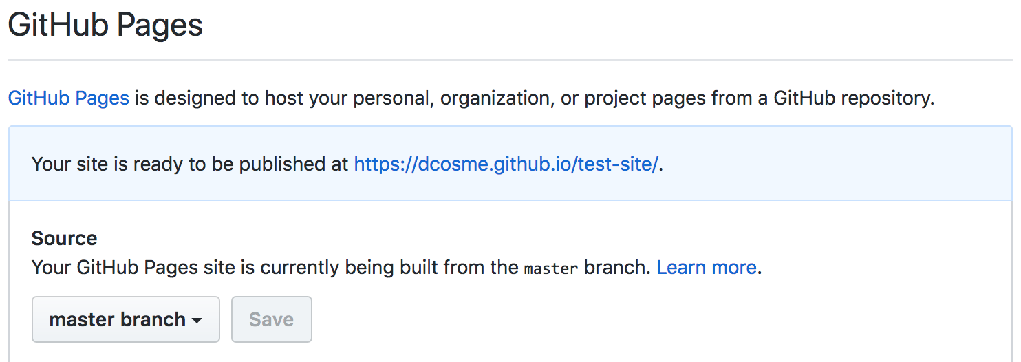
Go to your website and bask in the glory 🎉
Workflow
Here is the suggested workflow from the main developer of blogdown, Yihui Xie:
- Open your website project, click the “Serve Site” addin
- Revise old pages/posts, or click the “New Post” addin
- Write and save (take a look at the automatic preview)
- Push everything to Github, or upload the public/ directory to Netlify directly
More on the recommended workflow here.
Mini (mega? ulimate?) hack
You final hack in this class if to create a personal website and post it to GitHub. You can use any template you want or make it from scratch using the rmarkdown package (tutorial here).
Here are the components you should include:
- Homepage with a brief description about your research interests
- A CV (either written in markdown or simply uploaded as a PDF)
A “Resources” tab with at least one of your ‘contributions to science’ from this class.
Note: You decide how fancyyou want to be for #3. You may simply uploading your .html tutorial presentation. You can include the documentation and github link for the package you created last week. You can host a useful (or less useful) shiny app. You are limited only by your creativity (and your time).
Change colors, futz with custom CSS, make a shiny app and link to it – feel free to add anything else you’d like!
Go 🍌 🍌
Or just do the bare minimum because it’s the last week of the term 😄
Helpful resources
- https://bookdown.org/yihui/blogdown/
- https://apreshill.github.io/data-vis-labs-2018/slides/06-slides_blogdown.html#1
- https://alison.rbind.io/slides/blogdown-workshop-slides
- https://alison.rbind.io/post/up-and-running-with-blogdown/#build-your-site-in-rstudio
- http://amber.rbind.io/blog/2016/12/19/creatingsite/
- https://gohugo.io/
- http://elipapa.github.io/markdown-cv/