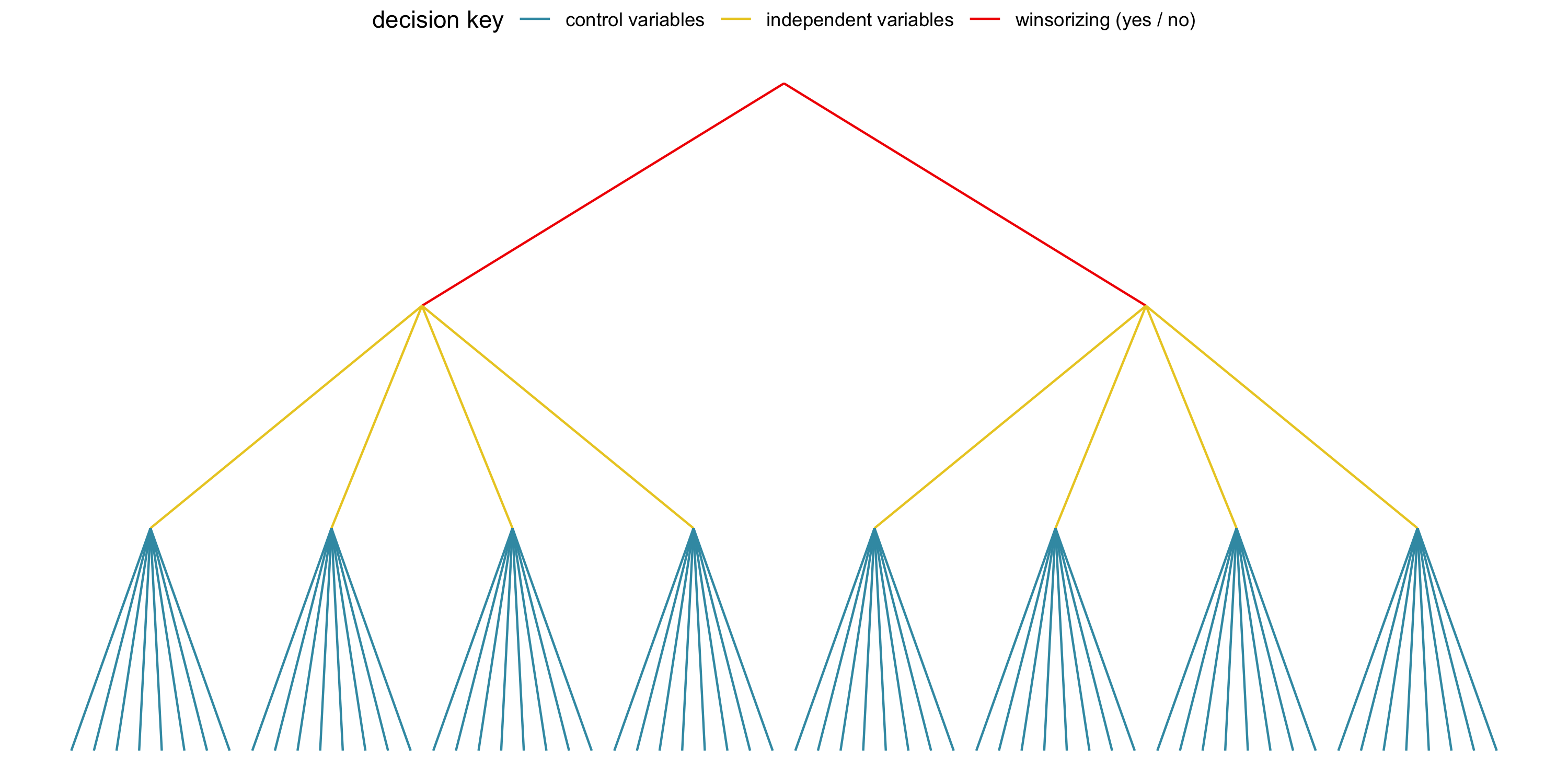
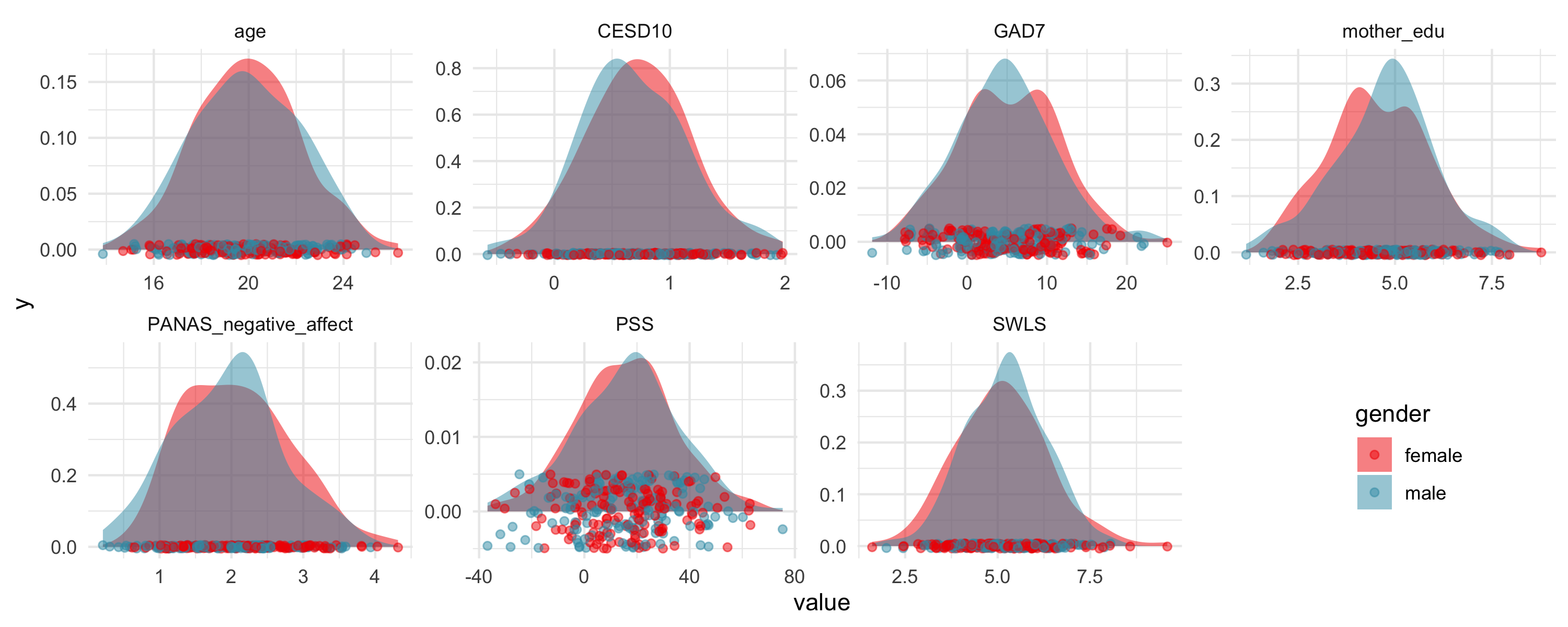
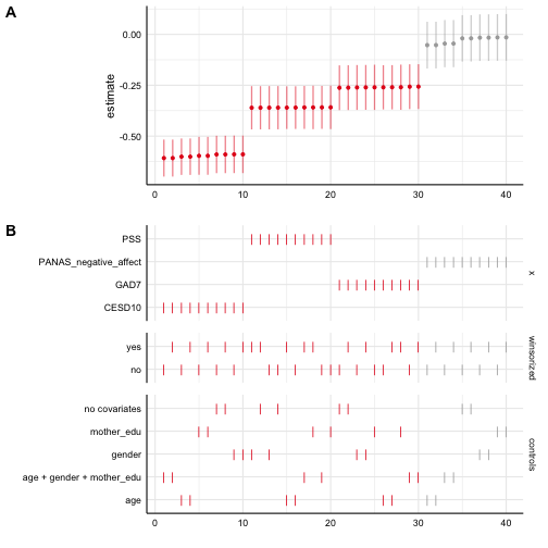
Specification Curve Analysis: A practical guide

class: center, middle, inverse, title-slide

# Specification Curve Analysis: A practical guide
## COMM 783 | University of Pennsylvania
### <a href="https://dcosme.github.io/">Dani Cosme</a>
### 2022-04-05

---

# The problem

There are many different ways to test a given association and we usually only report one or a few model specifications.

Model selection relies on choices by the researcher, and these choices are often arbitrary and sometimes driven by a desire for significant results.

Given the same dataset, two researchers might choose to answer the same question in very different ways.

Figure from [Simonsohn, Simmons, & Nelson, 2020](https://www.nature.com/articles/s41562-020-0912-z)

---

# The solution

According to [Simonsohn, Simmons, & Nelson, 2020](https://papers.ssrn.com/sol3/papers.cfm?abstract_id=2694998), the solution is to specify all "reasonable" models to test an association and assess the joint distribution across model specifications.

--
<br>

> Some researchers object to blindly running alternative specifications that may make little sense for theoretical or statistical reasons just for the sake of ‘robustness’. We are among those researchers. We believe one should test specifications that vary in as many of the potentially ad hoc assumptions as possible without testing any specifications that are not theoretically grounded.

--
<br>
This can be thought of as an explicit framework for sensitivity analyses / robustness checks, that enables inferential statistics across model specifications.

---

# Preregistration & SCA

---
# The value

A better understanding of how conceptual and analytic decisions alter the association of interest.

A more robust scientific literature with <span style="background-color: #21B0D4">increased generalizability and translational value</span>.

.center[
<img src="https://media.giphy.com/media/WUq1cg9K7uzHa/giphy.gif" width="50%" />
]

---

# SCA overview

--
### 1. Specify all reasonable models

### 2. Plot specification curve showing association/effect estimates as a function of decisions

### 3. Test how inconsistent the curve results are given the null hypothesis of no association/effect

---

## 1. Identify reasonable models
For the relationship of interest, determine the set of reasonable model specifications to test.

#### Reasonable specifications should be:
+ Consistent with theory
+ Expected to be statistically valid
+ Non-redundant

.center[
<img src="img/table1_2020.png" width="70%" />
]

Table from [Simonsohn, Simmons, & Nelson, 2020](https://www.nature.com/articles/s41562-020-0912-z)

---

## 1. Identify reasonable models

Del Guidice guidance

---
## 2. Descriptive specification curve
The specification curve visualizes the strength of the association/effect between two constructs of interest across model specifications and the analytic decisions associated with each model specification.

.pull-left[
**Key features**
* Two panels depicting 1) the curve and 2) the decisions
* A vertical slice = information about a single model specification
]

.pull-right[
<img src="https://media.springernature.com/full/springer-static/image/art%3A10.1038%2Fs41562-020-0912-z/MediaObjects/41562_2020_912_Fig2_HTML.png" width="100%" />

Figure from [Simonsohn, Simmons, & Nelson, 2020](https://www.nature.com/articles/s41562-020-0912-z)
]

---

## 2. Descriptive specification curve

#### The curve
* Model specifications are ranked

* Shows the model magnitude, sign (positive or negative), and statistical significance

* Often visualizes uncertainty around individual point estimates in the model specifications

* May highlight a single a priori or previously reported association/effect estimates

#### The decisions

* Each row denotes a specific decision and whether or not that decision applied to a given model specification

* Decisions are often grouped into categories to ease interpretation

---

## SCA examples

.panelset[
.panel[.panel-name[Simonsohn et al., 2020]
<img src="https://media.springernature.com/full/springer-static/image/art%3A10.1038%2Fs41562-020-0912-z/MediaObjects/41562_2020_912_Fig2_HTML.png" width="70%" style="display: block; margin: auto;" />

Figure from [Simonsohn, Simmons, & Nelson, 2020](https://www.nature.com/articles/s41562-020-0912-z)
]

.panel[.panel-name[Orben & Przybylski, 2019]
<img src="https://media.springernature.com/full/springer-static/image/art%3A10.1038%2Fs41562-018-0506-1/MediaObjects/41562_2018_506_Fig3_HTML.png" width="52%" style="display: block; margin: auto;" />

Example specification curve analysis (SCA) from [Orben  & Przybylski, 2019](http://nature.com/articles/s41562-018-0506-1)
]

.panel[.panel-name[Cosme & Lopez, 2020]
<img src="https://oup.silverchair-cdn.com/oup/backfile/Content_public/Journal/scan/PAP/10.1093_scan_nsaa155/2/nsaa155f1.jpeg?Expires=1652231337&Signature=bF-qwPQM2uk9U4ax9HcovP1UD5hfZarY7pDGZDfmV5cDwPYq~YWLDiHvpfoQtN0FwieSOYIMk1n5mLuS57oG36-atTuf9653INkwoEjrNge86E3dEqdzor~D3yhurWGE09vsuqLlm8M3TDr8IrFuujWzjFIGTWoVhxRW3zwt3cM1yzizhBTHZDmYCGInJXbQPQUFdrSYakpuRjTj8kj8RkkMWlnW4w3zRJrr0854Zvm4TobGS-IYDBTIRy9uBo35A9vt3h6-t2qWCC7tiTUi3xvIPxDiUIvOFFuLMO09~OdLSyFaMSpSxfwaD8fdKpaNfTlUPelvjsgdWkficjbIyQ__&Key-Pair-Id=APKAIE5G5CRDK6RD3PGA" width="57%" style="display: block; margin: auto;" />

Example specification curve analysis (SCA) from [Cosme & Lopez](https://psyarxiv.com/23mu5)
]

.panel[.panel-name[Cosme et al., preprint]
<br>
<img src="img/cosme_curve.png" width="35%" style="display: block; margin: auto;" />

Example specification curve analysis (SCA) from [Cosme et al., preprint](https://psyarxiv.com/9cxfj)
]
]

---

## 3. Inferential statistics
<br>
#### Metrics of interest in the observed curve

* Median curve estimate
* The share of positive or negative associations that are statistically significant

<br>
.center[
###But are the observed effects surprising given the null hypothesis?
]

---

## 3. Inferential statistics
#### Test inconsistency with the null

+ Use bootstrap resampling to create a distribution of curves under the null hypothesis

+ Experimental designs = shuffle the randomly assigned variable(s)
  
--

+ Observational designs = "force" the null by removing the effect of x on y for each observation and sample from this null dataset
  
--

+ Estimate the curve and extract the curve median, and share of positive/negative significant associations

+ Repeat many times to get a distribution

+ Compare observed curve metrics to null curves to generate p-values

---
## 3. Inferential statistics
#### Potential questions to test versus null

+ Is the median effect size in the observed curve statistically different than in the null distribution?

+ Is the share of dominant signs (e.g., positive or negative effects) that are statistically significant different than the null?

Table from [Simonsohn, Simmons, & Nelson, 2020](https://www.nature.com/articles/s41562-020-0912-z)

---
class: center, middle

# Tutorial

---

## 1. Define reasonable specifications

<br><br><br>
.center[
## What is the relationship between mental health
## and satisfaction with life?
]

---
## 1. Define reasonable specifications
--

#### Ways of operationalizing of the IV "mental health"
* `CEDS10` = depression score on the CESD-10
* `GAD` = anxiety score on the GAD-7
* `PANAS_negative_Affect` = negative affect score on the PANAS
* `PSS` = perceived stress score on the PSS

#### Control variables
* `age` = age
* `gender` = gender 
* `mother_edu` = maternal education

#### Analytic decisions
* Statistical modeling approach
  * Linear regression
* Outliers
  * Use all data points
  * Winsorize to the mean +/- 3 SD
  
---
## 1. Define reasonable specifications

### Visualize decisions
![](SCA_tutorial_inferential_presentation_files/figure-html/unnamed-chunk-10-1.png)

---

## Prep data
These data are generated based on an existing dataset from a study looking at health and well-being 
* Create winsorized independent variables (+/- 3 SD from the mean)
* Mean center and standardize each variable

.scroll-output[

```r
# load data
df = read.csv("sca_tutorial_inferences_data.csv", stringsAsFactors = FALSE)

# tidy for modeling
model_df = df %>%
  gather(variable, value, -PID, -age, -gender, -mother_edu, -SWLS) %>%
  group_by(variable) %>%
  mutate(mean_value = mean(value, na.rm = TRUE),
         sd3 = 3*sd(value, na.rm = TRUE)) %>%
  ungroup() %>%
  mutate(value_winsorized = ifelse(value > mean_value + sd3, mean_value + sd3,
                            ifelse(value < mean_value - sd3, mean_value - sd3, value)),
         variable_winsorized = sprintf("%s_winsorized", variable)) %>%
  select(-mean_value, -sd3) %>%
  spread(variable_winsorized, value_winsorized) %>%
  group_by(PID) %>%
  fill(contains("winsorized"), .direction = "downup") %>%
  spread(variable, value) %>%
  gather(variable, value, -PID, -age, -gender, -mother_edu) %>%
  group_by(variable) %>%
  mutate(value = scale(value, center = TRUE, scale = TRUE)) %>%
  spread(variable, value) %>%
  select(PID, age, gender, mother_edu, SWLS, sort(tidyselect::peek_vars()))

# print
# model_df %>%
#   mutate_if(is.numeric, ~round(., 2)) %>%
#   DT::datatable(rownames = FALSE, extensions = 'FixedColumns',
#                     options = list(scrollX = TRUE,
#                                    scrollY = TRUE,
#                                    pageLength = 5,
#                                    autoWidth = TRUE,
#                                    fixedColumns = list(leftColumns = 1),
#                                    dom = 't'))
```
]

---

## Plot distributions
![](SCA_tutorial_inferential_presentation_files/figure-html/unnamed-chunk-12-1.png)

---

## 2. Specify and estimate models

There are various methods for running a large number of model specifications.

Here, we unpack 3 different methods and discuss the advantages and disadvantages.

---

## estimate models using `MuMIn::dredge`

.panelset[
.panel[.panel-name[info]

#### Advantages
* Easily runs all nested models from a maximal model
* Provides model fit indices (e.g. AIC, BIC)

#### Disadvantages / limitations
* The max number of predictors = 30
* NAs must be omitted across all model specifications
* Doesn’t give parameter estimates for factors directly; you need to extract them using `MuMIn::get.models()`
* It may run nested models you aren't interested in if you don't subset
* If you have multiple independent variables of interest, you will need to specify each maximal model separately and combine after running
]

.panel[.panel-name[code]

```
## Fixed term is "(Intercept)"
```
]

.panel[.panel-name[output]
<div id="htmlwidget-1c9259eeb1ac673121b6" style="width:100%;height:auto;" class="datatables html-widget"></div>
<script type="application/json" data-for="htmlwidget-1c9259eeb1ac673121b6">{"x":{"filter":"none","vertical":false,"extensions":["FixedColumns"],"data":[[-1.75,-1.59,-1.76,-1.6,-0,0.15,-0.01,0.14,-1.44,-1.61,-1.49],[0.09,0.09,0.09,0.09,null,null,null,null,0.07,0.07,0.07],[-0.6,-0.61,-0.6,-0.61,-0.59,-0.6,-0.59,-0.6,null,null,null],[null,null,"+","+",null,null,"+","+",null,null,"+"],[null,-0.04,null,-0.04,null,-0.03,null,-0.03,null,0.04,null],[726.82,731.46,732.44,737.04,739.02,743.9,744.67,749.51,859.63,864.62,864.8],[4,5,5,6,3,4,4,5,3,4,4],[-352,-351.47,-351.96,-351.41,-360.96,-360.54,-360.93,-360.5,-421.26,-420.9,-420.99],[712.01,712.94,713.92,714.82,727.91,729.08,729.85,731,848.52,849.8,849.99],[0,0.93,1.91,2.81,15.91,17.07,17.85,18.99,136.51,137.79,137.98],[0.442659571448505,0.278050016474999,0.170340778996004,0.10861407605703,0.000156109282660448,8.69693964534258e-05,5.91783811470632e-05,3.32999631995666e-05,1.00762746576532e-30,5.31314328955758e-31,4.83162870447504e-31]],"container":"<table class=\"display\">\n  <thead>\n    <tr>\n      <th>(Intercept)<\/th>\n      <th>age<\/th>\n      <th>CESD10<\/th>\n      <th>gender<\/th>\n      <th>mother_edu<\/th>\n      <th>BIC<\/th>\n      <th>df<\/th>\n      <th>logLik<\/th>\n      <th>AIC<\/th>\n      <th>delta<\/th>\n      <th>weight<\/th>\n    <\/tr>\n  <\/thead>\n<\/table>","options":{"scrollX":true,"scrollY":true,"pageLength":5,"autoWidth":true,"dom":"t","columnDefs":[{"className":"dt-right","targets":[0,1,2,4,5,6,7,8,9,10]}],"order":[],"orderClasses":false,"lengthMenu":[5,10,25,50,100]}},"evals":[],"jsHooks":[]}</script>
]
]

---

## estimate models using `purrr`

.panelset[
.panel[.panel-name[info]

#### Advantages
* Greater control over how models are specified

#### Disadvantages / limitations
* Need to code from scratch

Note that if you are running linear mixed effects models, you can use the `broom.mixed` instead of the `broom` package to tidy the model output.
]

.panel[.panel-name[code]

]

.panel[.panel-name[output]
<div id="htmlwidget-c7a189b83021a1bf3f23" style="width:100%;height:auto;" class="datatables html-widget"></div>
<script type="application/json" data-for="htmlwidget-c7a189b83021a1bf3f23">{"x":{"filter":"none","vertical":false,"extensions":["FixedColumns"],"data":[["SWLS ~ CESD10 + age","SWLS ~ CESD10_winsorized + age","SWLS ~ GAD7 + age","SWLS ~ GAD7_winsorized + age","SWLS ~ PANAS_negative_affect + age","SWLS ~ PANAS_negative_affect_winsorized + age","SWLS ~ PSS + age","SWLS ~ PSS_winsorized + age","SWLS ~ CESD10 + gender","SWLS ~ CESD10_winsorized + gender","SWLS ~ GAD7 + gender","SWLS ~ GAD7_winsorized + gender","SWLS ~ PANAS_negative_affect + gender","SWLS ~ PANAS_negative_affect_winsorized + gender","SWLS ~ PSS + gender","SWLS ~ PSS_winsorized + gender","SWLS ~ CESD10 + mother_edu","SWLS ~ CESD10_winsorized + mother_edu","SWLS ~ GAD7 + mother_edu","SWLS ~ GAD7_winsorized + mother_edu","SWLS ~ PANAS_negative_affect + mother_edu","SWLS ~ PANAS_negative_affect_winsorized + mother_edu","SWLS ~ PSS + mother_edu","SWLS ~ PSS_winsorized + mother_edu","SWLS ~ CESD10 + age + gender","SWLS ~ CESD10_winsorized + age + gender","SWLS ~ GAD7 + age + gender","SWLS ~ GAD7_winsorized + age + gender","SWLS ~ PANAS_negative_affect + age + gender","SWLS ~ PANAS_negative_affect_winsorized + age + gender","SWLS ~ PSS + age + gender","SWLS ~ PSS_winsorized + age + gender","SWLS ~ CESD10 + age + mother_edu","SWLS ~ CESD10_winsorized + age + mother_edu","SWLS ~ GAD7 + age + mother_edu","SWLS ~ GAD7_winsorized + age + mother_edu","SWLS ~ PANAS_negative_affect + age + mother_edu","SWLS ~ PANAS_negative_affect_winsorized + age + mother_edu","SWLS ~ PSS + age + mother_edu","SWLS ~ PSS_winsorized + age + mother_edu","SWLS ~ CESD10 + gender + mother_edu","SWLS ~ CESD10_winsorized + gender + mother_edu","SWLS ~ GAD7 + gender + mother_edu","SWLS ~ GAD7_winsorized + gender + mother_edu","SWLS ~ PANAS_negative_affect + gender + mother_edu","SWLS ~ PANAS_negative_affect_winsorized + gender + mother_edu","SWLS ~ PSS + gender + mother_edu","SWLS ~ PSS_winsorized + gender + mother_edu","SWLS ~ CESD10 + age + gender + mother_edu","SWLS ~ CESD10_winsorized + age + gender + mother_edu","SWLS ~ GAD7 + age + gender + mother_edu","SWLS ~ GAD7_winsorized + age + gender + mother_edu","SWLS ~ PANAS_negative_affect + age + gender + mother_edu","SWLS ~ PANAS_negative_affect_winsorized + age + gender + mother_edu","SWLS ~ PSS + age + gender + mother_edu","SWLS ~ PSS_winsorized + age + gender + mother_edu","SWLS ~ CESD10","SWLS ~ CESD10_winsorized","SWLS ~ GAD7","SWLS ~ GAD7_winsorized","SWLS ~ PANAS_negative_affect","SWLS ~ PANAS_negative_affect_winsorized","SWLS ~ PSS","SWLS ~ PSS_winsorized"],["lm","lm","lm","lm","lm","lm","lm","lm","lm","lm","lm","lm","lm","lm","lm","lm","lm","lm","lm","lm","lm","lm","lm","lm","lm","lm","lm","lm","lm","lm","lm","lm","lm","lm","lm","lm","lm","lm","lm","lm","lm","lm","lm","lm","lm","lm","lm","lm","lm","lm","lm","lm","lm","lm","lm","lm","lm","lm","lm","lm","lm","lm","lm","lm"],["SWLS","SWLS","SWLS","SWLS","SWLS","SWLS","SWLS","SWLS","SWLS","SWLS","SWLS","SWLS","SWLS","SWLS","SWLS","SWLS","SWLS","SWLS","SWLS","SWLS","SWLS","SWLS","SWLS","SWLS","SWLS","SWLS","SWLS","SWLS","SWLS","SWLS","SWLS","SWLS","SWLS","SWLS","SWLS","SWLS","SWLS","SWLS","SWLS","SWLS","SWLS","SWLS","SWLS","SWLS","SWLS","SWLS","SWLS","SWLS","SWLS","SWLS","SWLS","SWLS","SWLS","SWLS","SWLS","SWLS","SWLS","SWLS","SWLS","SWLS","SWLS","SWLS","SWLS","SWLS"],["CESD10","CESD10_winsorized","GAD7","GAD7_winsorized","PANAS_negative_affect","PANAS_negative_affect_winsorized","PSS","PSS_winsorized","CESD10","CESD10_winsorized","GAD7","GAD7_winsorized","PANAS_negative_affect","PANAS_negative_affect_winsorized","PSS","PSS_winsorized","CESD10","CESD10_winsorized","GAD7","GAD7_winsorized","PANAS_negative_affect","PANAS_negative_affect_winsorized","PSS","PSS_winsorized","CESD10","CESD10_winsorized","GAD7","GAD7_winsorized","PANAS_negative_affect","PANAS_negative_affect_winsorized","PSS","PSS_winsorized","CESD10","CESD10_winsorized","GAD7","GAD7_winsorized","PANAS_negative_affect","PANAS_negative_affect_winsorized","PSS","PSS_winsorized","CESD10","CESD10_winsorized","GAD7","GAD7_winsorized","PANAS_negative_affect","PANAS_negative_affect_winsorized","PSS","PSS_winsorized","CESD10","CESD10_winsorized","GAD7","GAD7_winsorized","PANAS_negative_affect","PANAS_negative_affect_winsorized","PSS","PSS_winsorized","CESD10","CESD10_winsorized","GAD7","GAD7_winsorized","PANAS_negative_affect","PANAS_negative_affect_winsorized","PSS","PSS_winsorized"],["age","age","age","age","age","age","age","age","gender","gender","gender","gender","gender","gender","gender","gender","mother_edu","mother_edu","mother_edu","mother_edu","mother_edu","mother_edu","mother_edu","mother_edu","age + gender","age + gender","age + gender","age + gender","age + gender","age + gender","age + gender","age + gender","age + mother_edu","age + mother_edu","age + mother_edu","age + mother_edu","age + mother_edu","age + mother_edu","age + mother_edu","age + mother_edu","gender + mother_edu","gender + mother_edu","gender + mother_edu","gender + mother_edu","gender + mother_edu","gender + mother_edu","gender + mother_edu","gender + mother_edu","age + gender + mother_edu","age + gender + mother_edu","age + gender + mother_edu","age + gender + mother_edu","age + gender + mother_edu","age + gender + mother_edu","age + gender + mother_edu","age + gender + mother_edu","no covariates","no covariates","no covariates","no covariates","no covariates","no covariates","no covariates","no covariates"],[-0.6,-0.6,-0.26,-0.26,-0.05,-0.05,-0.36,-0.36,-0.59,-0.59,-0.26,-0.26,-0.02,-0.02,-0.36,-0.36,-0.6,-0.6,-0.26,-0.26,-0.01,-0.01,-0.36,-0.36,-0.6,-0.6,-0.26,-0.26,-0.05,-0.05,-0.36,-0.36,-0.61,-0.61,-0.26,-0.26,-0.05,-0.05,-0.36,-0.36,-0.6,-0.6,-0.26,-0.26,-0.01,-0.01,-0.36,-0.36,-0.61,-0.61,-0.26,-0.26,-0.05,-0.05,-0.36,-0.36,-0.59,-0.59,-0.26,-0.26,-0.02,-0.02,-0.36,-0.36],[0.05,0.05,0.06,0.06,0.06,0.06,0.05,0.05,0.05,0.05,0.06,0.06,0.06,0.06,0.05,0.05,0.05,0.05,0.06,0.06,0.06,0.06,0.05,0.05,0.05,0.05,0.06,0.06,0.06,0.06,0.05,0.05,0.05,0.05,0.06,0.06,0.06,0.06,0.05,0.05,0.05,0.05,0.06,0.06,0.06,0.06,0.05,0.05,0.05,0.05,0.06,0.06,0.06,0.06,0.05,0.05,0.05,0.05,0.06,0.06,0.06,0.06,0.05,0.05],[-13.2,-13.2,-4.71,-4.7,-0.91,-0.9,-6.75,-6.75,-12.57,-12.57,-4.66,-4.65,-0.28,-0.28,-6.66,-6.67,-12.6,-12.6,-4.61,-4.6,-0.26,-0.25,-6.6,-6.61,-13.15,-13.15,-4.67,-4.66,-0.85,-0.84,-6.75,-6.75,-13.2,-13.2,-4.63,-4.62,-0.83,-0.82,-6.68,-6.69,-12.56,-12.56,-4.58,-4.57,-0.21,-0.2,-6.6,-6.61,-13.16,-13.16,-4.59,-4.59,-0.77,-0.77,-6.68,-6.69,-12.62,-12.62,-4.69,-4.68,-0.34,-0.33,-6.67,-6.67],[0,0,0,0,0.37,0.37,0,0,0,0,0,0,0.78,0.78,0,0,0,0,0,0,0.8,0.8,0,0,0,0,0,0,0.4,0.4,0,0,0,0,0,0,0.41,0.41,0,0,0,0,0,0,0.84,0.84,0,0,0,0,0,0,0.44,0.44,0,0,0,0,0,0,0.74,0.74,0,0],[-0.69,-0.69,-0.37,-0.37,-0.17,-0.17,-0.46,-0.47,-0.68,-0.68,-0.37,-0.37,-0.13,-0.13,-0.47,-0.47,-0.69,-0.69,-0.37,-0.37,-0.13,-0.13,-0.47,-0.47,-0.69,-0.69,-0.37,-0.37,-0.16,-0.16,-0.46,-0.47,-0.7,-0.7,-0.37,-0.37,-0.16,-0.16,-0.46,-0.46,-0.69,-0.69,-0.37,-0.37,-0.13,-0.13,-0.47,-0.47,-0.7,-0.7,-0.37,-0.37,-0.16,-0.16,-0.46,-0.46,-0.68,-0.68,-0.37,-0.37,-0.13,-0.13,-0.47,-0.47],[-0.51,-0.51,-0.15,-0.15,0.06,0.06,-0.25,-0.26,-0.5,-0.5,-0.15,-0.15,0.1,0.1,-0.25,-0.25,-0.5,-0.5,-0.15,-0.15,0.1,0.1,-0.25,-0.25,-0.51,-0.51,-0.15,-0.15,0.07,0.07,-0.25,-0.26,-0.52,-0.52,-0.15,-0.15,0.07,0.07,-0.25,-0.25,-0.5,-0.5,-0.15,-0.15,0.1,0.1,-0.25,-0.25,-0.52,-0.52,-0.15,-0.15,0.07,0.07,-0.25,-0.25,-0.5,-0.5,-0.15,-0.15,0.09,0.09,-0.25,-0.25],[300,300,300,300,300,300,300,300,300,300,300,300,300,300,300,300,300,300,300,300,300,300,300,300,300,300,300,300,300,300,300,300,300,300,300,300,300,300,300,300,300,300,300,300,300,300,300,300,300,300,300,300,300,300,300,300,300,300,300,300,300,300,300,300]],"container":"<table class=\"display\">\n  <thead>\n    <tr>\n      <th>formula<\/th>\n      <th>model<\/th>\n      <th>y<\/th>\n      <th>x<\/th>\n      <th>controls<\/th>\n      <th>estimate<\/th>\n      <th>std.error<\/th>\n      <th>statistic<\/th>\n      <th>p.value<\/th>\n      <th>conf.low<\/th>\n      <th>conf.high<\/th>\n      <th>obs<\/th>\n    <\/tr>\n  <\/thead>\n<\/table>","options":{"scrollX":true,"scrollY":true,"pageLength":5,"autoWidth":true,"dom":"t","columnDefs":[{"className":"dt-right","targets":[5,6,7,8,9,10,11]}],"order":[],"orderClasses":false,"lengthMenu":[5,10,25,50,100]}},"evals":[],"jsHooks":[]}</script>
]
]

---

## estimate models using `specr`

.panelset[
.panel[.panel-name[info]

#### Advantages
* Very simple to use!
* You can easily run the models in specific subsets of your data

#### Disadvantages / limitations
* <controls>
]

.panel[.panel-name[code]

]

.panel[.panel-name[output]
<div id="htmlwidget-e68b10c131afa429a851" style="width:100%;height:auto;" class="datatables html-widget"></div>
<script type="application/json" data-for="htmlwidget-e68b10c131afa429a851">{"x":{"filter":"none","vertical":false,"extensions":["FixedColumns"],"data":[["CESD10","CESD10_winsorized","GAD7","GAD7_winsorized","PANAS_negative_affect","PANAS_negative_affect_winsorized","PSS","PSS_winsorized","CESD10","CESD10_winsorized","GAD7","GAD7_winsorized","PANAS_negative_affect","PANAS_negative_affect_winsorized","PSS","PSS_winsorized","CESD10","CESD10_winsorized","GAD7","GAD7_winsorized","PANAS_negative_affect","PANAS_negative_affect_winsorized","PSS","PSS_winsorized","CESD10","CESD10_winsorized","GAD7","GAD7_winsorized","PANAS_negative_affect","PANAS_negative_affect_winsorized","PSS","PSS_winsorized","CESD10","CESD10_winsorized","GAD7","GAD7_winsorized","PANAS_negative_affect","PANAS_negative_affect_winsorized","PSS","PSS_winsorized"],["SWLS","SWLS","SWLS","SWLS","SWLS","SWLS","SWLS","SWLS","SWLS","SWLS","SWLS","SWLS","SWLS","SWLS","SWLS","SWLS","SWLS","SWLS","SWLS","SWLS","SWLS","SWLS","SWLS","SWLS","SWLS","SWLS","SWLS","SWLS","SWLS","SWLS","SWLS","SWLS","SWLS","SWLS","SWLS","SWLS","SWLS","SWLS","SWLS","SWLS"],["lm","lm","lm","lm","lm","lm","lm","lm","lm","lm","lm","lm","lm","lm","lm","lm","lm","lm","lm","lm","lm","lm","lm","lm","lm","lm","lm","lm","lm","lm","lm","lm","lm","lm","lm","lm","lm","lm","lm","lm"],["age + gender + mother_edu","age + gender + mother_edu","age + gender + mother_edu","age + gender + mother_edu","age + gender + mother_edu","age + gender + mother_edu","age + gender + mother_edu","age + gender + mother_edu","age","age","age","age","age","age","age","age","gender","gender","gender","gender","gender","gender","gender","gender","mother_edu","mother_edu","mother_edu","mother_edu","mother_edu","mother_edu","mother_edu","mother_edu","no covariates","no covariates","no covariates","no covariates","no covariates","no covariates","no covariates","no covariates"],[-0.61,-0.61,-0.26,-0.26,-0.05,-0.05,-0.36,-0.36,-0.6,-0.6,-0.26,-0.26,-0.05,-0.05,-0.36,-0.36,-0.59,-0.59,-0.26,-0.26,-0.02,-0.02,-0.36,-0.36,-0.6,-0.6,-0.26,-0.26,-0.01,-0.01,-0.36,-0.36,-0.59,-0.59,-0.26,-0.26,-0.02,-0.02,-0.36,-0.36],[0.05,0.05,0.06,0.06,0.06,0.06,0.05,0.05,0.05,0.05,0.06,0.06,0.06,0.06,0.05,0.05,0.05,0.05,0.06,0.06,0.06,0.06,0.05,0.05,0.05,0.05,0.06,0.06,0.06,0.06,0.05,0.05,0.05,0.05,0.06,0.06,0.06,0.06,0.05,0.05],[-13.16,-13.16,-4.59,-4.59,-0.77,-0.77,-6.68,-6.69,-13.2,-13.2,-4.71,-4.7,-0.91,-0.9,-6.75,-6.75,-12.57,-12.57,-4.66,-4.65,-0.28,-0.28,-6.66,-6.67,-12.6,-12.6,-4.61,-4.6,-0.26,-0.25,-6.6,-6.61,-12.62,-12.62,-4.69,-4.68,-0.34,-0.33,-6.67,-6.67],[0,0,0,0,0.44,0.44,0,0,0,0,0,0,0.37,0.37,0,0,0,0,0,0,0.78,0.78,0,0,0,0,0,0,0.8,0.8,0,0,0,0,0,0,0.74,0.74,0,0],[-0.7,-0.7,-0.37,-0.37,-0.16,-0.16,-0.46,-0.46,-0.69,-0.69,-0.37,-0.37,-0.17,-0.17,-0.46,-0.47,-0.68,-0.68,-0.37,-0.37,-0.13,-0.13,-0.47,-0.47,-0.69,-0.69,-0.37,-0.37,-0.13,-0.13,-0.47,-0.47,-0.68,-0.68,-0.37,-0.37,-0.13,-0.13,-0.47,-0.47],[-0.52,-0.52,-0.15,-0.15,0.07,0.07,-0.25,-0.25,-0.51,-0.51,-0.15,-0.15,0.06,0.06,-0.25,-0.26,-0.5,-0.5,-0.15,-0.15,0.1,0.1,-0.25,-0.25,-0.5,-0.5,-0.15,-0.15,0.1,0.1,-0.25,-0.25,-0.5,-0.5,-0.15,-0.15,0.09,0.09,-0.25,-0.25],[0.39,0.39,0.09,0.09,0.03,0.03,0.16,0.16,0.39,0.39,0.09,0.09,0.03,0.03,0.16,0.16,0.35,0.35,0.07,0.07,0,0,0.13,0.13,0.35,0.35,0.07,0.07,0,0,0.13,0.13,0.35,0.35,0.07,0.07,0,0,0.13,0.13],[0.38,0.38,0.08,0.08,0.02,0.02,0.15,0.15,0.38,0.38,0.09,0.09,0.02,0.02,0.15,0.15,0.34,0.34,0.06,0.06,-0,-0,0.13,0.13,0.35,0.35,0.06,0.06,-0,-0,0.12,0.12,0.35,0.35,0.07,0.07,-0,-0,0.13,0.13],[0.79,0.79,0.96,0.96,0.99,0.99,0.92,0.92,0.79,0.79,0.96,0.96,0.99,0.99,0.92,0.92,0.81,0.81,0.97,0.97,1,1,0.94,0.93,0.81,0.81,0.97,0.97,1,1,0.94,0.94,0.81,0.81,0.97,0.97,1,1,0.93,0.93],[46.85,46.85,7.69,7.68,2.41,2.41,13.77,13.78,93.38,93.38,15.31,15.28,4.35,4.35,27.3,27.33,79.41,79.41,11.09,11.05,0.27,0.27,22.47,22.51,80,80,11.01,10.98,0.41,0.41,22.21,22.25,159.26,159.26,22.02,21.94,0.11,0.11,44.43,44.53],[0,0,0,0,0.05,0.05,0,0,0,0,0,0,0.01,0.01,0,0,0,0,0,0,0.76,0.76,0,0,0,0,0,0,0.66,0.66,0,0,0,0,0,0,0.74,0.74,0,0],[4,4,4,4,4,4,4,4,2,2,2,2,2,2,2,2,2,2,2,2,2,2,2,2,2,2,2,2,2,2,2,2,1,1,1,1,1,1,1,1],[-351.41,-351.41,-410.3,-410.33,-420.36,-420.37,-399.51,-399.48,-352,-352,-410.46,-410.49,-420.85,-420.85,-399.87,-399.84,-360.93,-360.93,-414.38,-414.41,-424.91,-424.91,-404.05,-404.01,-360.54,-360.54,-414.45,-414.48,-424.77,-424.77,-404.28,-404.24,-360.96,-360.96,-414.49,-414.52,-425.12,-425.12,-404.33,-404.29],[714.82,714.82,832.6,832.66,852.73,852.73,811.02,810.96,712.01,712.01,828.92,828.98,849.69,849.7,807.74,807.68,729.85,729.85,836.76,836.82,857.81,857.82,816.09,816.01,729.08,729.08,836.9,836.97,857.53,857.54,816.55,816.47,727.91,727.91,834.98,835.05,856.25,856.25,814.67,814.58],[737.04,737.04,854.83,854.88,874.95,874.96,833.24,833.18,726.82,726.82,843.73,843.79,864.51,864.51,822.56,822.49,744.67,744.67,851.57,851.64,872.63,872.63,830.91,830.83,743.9,743.9,851.71,851.78,872.35,872.35,831.37,831.29,739.02,739.02,846.09,846.16,867.36,867.36,825.78,825.7],[182.84,182.84,270.76,270.82,289.55,289.56,251.97,251.92,183.57,183.57,271.05,271.1,290.48,290.49,252.57,252.52,194.82,194.82,278.23,278.29,298.45,298.46,259.71,259.64,194.32,194.32,278.35,278.42,298.18,298.18,260.1,260.03,194.86,194.86,278.43,278.49,298.89,298.89,260.2,260.13],[295,295,295,295,295,295,295,295,297,297,297,297,297,297,297,297,297,297,297,297,297,297,297,297,297,297,297,297,297,297,297,297,298,298,298,298,298,298,298,298],[300,300,300,300,300,300,300,300,300,300,300,300,300,300,300,300,300,300,300,300,300,300,300,300,300,300,300,300,300,300,300,300,300,300,300,300,300,300,300,300],["all","all","all","all","all","all","all","all","all","all","all","all","all","all","all","all","all","all","all","all","all","all","all","all","all","all","all","all","all","all","all","all","all","all","all","all","all","all","all","all"]],"container":"<table class=\"display\">\n  <thead>\n    <tr>\n      <th>x<\/th>\n      <th>y<\/th>\n      <th>model<\/th>\n      <th>controls<\/th>\n      <th>estimate<\/th>\n      <th>std.error<\/th>\n      <th>statistic<\/th>\n      <th>p.value<\/th>\n      <th>conf.low<\/th>\n      <th>conf.high<\/th>\n      <th>fit_r.squared<\/th>\n      <th>fit_adj.r.squared<\/th>\n      <th>fit_sigma<\/th>\n      <th>fit_statistic<\/th>\n      <th>fit_p.value<\/th>\n      <th>fit_df<\/th>\n      <th>fit_logLik<\/th>\n      <th>fit_AIC<\/th>\n      <th>fit_BIC<\/th>\n      <th>fit_deviance<\/th>\n      <th>fit_df.residual<\/th>\n      <th>fit_nobs<\/th>\n      <th>subsets<\/th>\n    <\/tr>\n  <\/thead>\n<\/table>","options":{"scrollX":true,"scrollY":true,"pageLength":5,"autoWidth":true,"dom":"t","columnDefs":[{"className":"dt-right","targets":[4,5,6,7,8,9,10,11,12,13,14,15,16,17,18,19,20,21]}],"order":[],"orderClasses":false,"lengthMenu":[5,10,25,50,100]}},"evals":[],"jsHooks":[]}</script>
]
]

---

## 3. Plot specification curve

### Guide to unpacking the curve
Panel A
* X-axis = ordered model specifications
* Y-axis = standardized regression coefficient for the IV-DV relationship 
* Points = the standardized regression coefficient for a specific models
* Error bars = 95% confidence intervals around the point estimate

Panel B
* X-axis = ordered model specifications (the same as panel A)
* Y-axis (right) = analytic decision categories
* Y-axis (left) = specific analytic decisions within each category
* Lines = denote that a specific analytic decision was true for that model specification

Color key
* Red = regression coefficient was statistically significant values at p < .05
* Black/grey = regression coefficient was p > .05

---

## Homebrew SCA plot with `purrr` output
.panelset[
.panel[.panel-name[code]

```r
# set plot aesthetics
aes = theme_minimal(base_size = 11) +
      theme(legend.title = element_text(size = 10),
          legend.text = element_text(size = 9),
          axis.text = element_text(color = "black"),
          axis.line = element_line(colour = "black"),
          legend.position = "none",
          panel.border = element_blank(),
          panel.background = element_blank())

colors = c("yes" = "#F21A00", "no" = "black")

# merge and tidy for plotting
plot_data = output_purrr %>%
  arrange(estimate) %>%
  mutate(specification = row_number(),
         winsorized = ifelse(grepl("winsorized", x), "yes", "no"),
         significant.p = ifelse(p.value < .05, "yes", "no"),
         x = gsub("_winsorized", "", x))

# plot top panel
top = plot_data %>%
  ggplot(aes(specification, estimate, color = significant.p)) +
    geom_pointrange(aes(ymin = conf.low, ymax = conf.high), size = .25, shape = "", alpha = .5) +
    geom_point(size = .5) +
    scale_color_manual(values = colors) + 
    labs(x = "", y = "standardized\nregression coefficient\n") + 
    aes

# rename variables and plot bottom panel
for (var in c(control_vars, "no covariates")) {
  plot_data = plot_data %>%
    mutate(!!var :=  ifelse(grepl(var, controls), "yes", "no"))
}

bottom = plot_data %>%
  gather(controls, control_value, eval(control_vars), `no covariates`) %>% 
  gather(variable, value, x, controls, winsorized) %>%
  filter(control_value == "yes") %>%
  unique() %>%
  mutate(variable = factor(variable, levels = c("x", "winsorized", "controls"))) %>% 
  ggplot(aes(x = specification,
             y = value,
             color = significant.p)) +
    geom_point(aes(x = specification,
                   y = value),
               shape = 124,
               size = 3) +
    facet_grid(variable ~ 1, scales = "free_y", space = "free_y") +
    scale_color_manual(values = colors) + 
    labs(x = "\nspecification number", y = "") + 
    aes +
    theme(strip.text.x = element_blank())
```
]

.panel[.panel-name[output]
<img src="SCA_tutorial_inferential_presentation_files/figure-html/unnamed-chunk-16-1.png" width="360" style="display: block; margin: auto;" />
]
]

---

## SCA plot with `specr`

.panelset[
.panel[.panel-name[code]

```r
output_specr %>%
  mutate(winsorized = ifelse(grepl("winsorized", x), "yes", "no"),
         x = gsub("_winsorized", "", x)) %>%
  plot_specs(., choices = c("x", "winsorized", "controls"))
```

![](SCA_tutorial_inferential_presentation_files/figure-html/unnamed-chunk-17-1.png)
]
.panel[.panel-name[output]
<img src="SCA_tutorial_inferential_presentation_files/figure-html/unnamed-chunk-18-1.png" width="360" style="display: block; margin: auto;" />
]
]

---

## 4. Inferential statistics

1. Run the SCA and extract the median, and the number of positive and negative statistically significant models

2. Use bootstrap resampling to create a distribution of curves under the null hypothesis

3. Generate p-values indicating how surprising the observed results are under the null hypothesis

---

## Null boostrap resampling

.panelset[
.panel[.panel-name[overview]

* Run SCA to retrieve associations between the independent and dependent variable in each model specification

* Extract the dataset for each model specification (which was saved as a model object `fit` in the data frame)

* Force the null on each specification by subtracting the effect of the independent variable of interest (b estimate * x) from the dependent variable (y_value) for each observation in the dataset

* For each bootstrap, sample with replacement from the null dataset and run all model specifications to generate a curve

* Extract median estimate, N positive & significant at p < .05, and N negative & significant p < .05

* Repeat process many times (e.g. 500 or 1000)

]
.panel[.panel-name[define functions]
`run_boot_null` = wrapper function to run the bootstrapping procedure or load an existing output file

`sca_boot_null` = function that runs the boostrapping procedure

`summarize_sca` = function to summarize the observed specification curve

`summarize_boot_null` = function to summarize the bootstrapped curves

]
.panel[.panel-name[bootstrap `specr` output]

<div id="htmlwidget-45fe5e73cbc3e75810a6" style="width:100%;height:auto;" class="datatables html-widget"></div>
<script type="application/json" data-for="htmlwidget-45fe5e73cbc3e75810a6">{"x":{"filter":"none","vertical":false,"extensions":["FixedColumns"],"data":[["Bootstrap001","Bootstrap002","Bootstrap003","Bootstrap004","Bootstrap005","Bootstrap006","Bootstrap007","Bootstrap008","Bootstrap009","Bootstrap010","Bootstrap011","Bootstrap012","Bootstrap013","Bootstrap014","Bootstrap015","Bootstrap016","Bootstrap017","Bootstrap018","Bootstrap019","Bootstrap020","Bootstrap021","Bootstrap022","Bootstrap023","Bootstrap024","Bootstrap025","Bootstrap026","Bootstrap027","Bootstrap028","Bootstrap029","Bootstrap030","Bootstrap031","Bootstrap032","Bootstrap033","Bootstrap034","Bootstrap035","Bootstrap036","Bootstrap037","Bootstrap038","Bootstrap039","Bootstrap040","Bootstrap041","Bootstrap042","Bootstrap043","Bootstrap044","Bootstrap045","Bootstrap046","Bootstrap047","Bootstrap048","Bootstrap049","Bootstrap050","Bootstrap051","Bootstrap052","Bootstrap053","Bootstrap054","Bootstrap055","Bootstrap056","Bootstrap057","Bootstrap058","Bootstrap059","Bootstrap060","Bootstrap061","Bootstrap062","Bootstrap063","Bootstrap064","Bootstrap065","Bootstrap066","Bootstrap067","Bootstrap068","Bootstrap069","Bootstrap070","Bootstrap071","Bootstrap072","Bootstrap073","Bootstrap074","Bootstrap075","Bootstrap076","Bootstrap077","Bootstrap078","Bootstrap079","Bootstrap080","Bootstrap081","Bootstrap082","Bootstrap083","Bootstrap084","Bootstrap085","Bootstrap086","Bootstrap087","Bootstrap088","Bootstrap089","Bootstrap090","Bootstrap091","Bootstrap092","Bootstrap093","Bootstrap094","Bootstrap095","Bootstrap096","Bootstrap097","Bootstrap098","Bootstrap099","Bootstrap100","Bootstrap101","Bootstrap102","Bootstrap103","Bootstrap104","Bootstrap105","Bootstrap106","Bootstrap107","Bootstrap108","Bootstrap109","Bootstrap110","Bootstrap111","Bootstrap112","Bootstrap113","Bootstrap114","Bootstrap115","Bootstrap116","Bootstrap117","Bootstrap118","Bootstrap119","Bootstrap120","Bootstrap121","Bootstrap122","Bootstrap123","Bootstrap124","Bootstrap125","Bootstrap126","Bootstrap127","Bootstrap128","Bootstrap129","Bootstrap130","Bootstrap131","Bootstrap132","Bootstrap133","Bootstrap134","Bootstrap135","Bootstrap136","Bootstrap137","Bootstrap138","Bootstrap139","Bootstrap140","Bootstrap141","Bootstrap142","Bootstrap143","Bootstrap144","Bootstrap145","Bootstrap146","Bootstrap147","Bootstrap148","Bootstrap149","Bootstrap150","Bootstrap151","Bootstrap152","Bootstrap153","Bootstrap154","Bootstrap155","Bootstrap156","Bootstrap157","Bootstrap158","Bootstrap159","Bootstrap160","Bootstrap161","Bootstrap162","Bootstrap163","Bootstrap164","Bootstrap165","Bootstrap166","Bootstrap167","Bootstrap168","Bootstrap169","Bootstrap170","Bootstrap171","Bootstrap172","Bootstrap173","Bootstrap174","Bootstrap175","Bootstrap176","Bootstrap177","Bootstrap178","Bootstrap179","Bootstrap180","Bootstrap181","Bootstrap182","Bootstrap183","Bootstrap184","Bootstrap185","Bootstrap186","Bootstrap187","Bootstrap188","Bootstrap189","Bootstrap190","Bootstrap191","Bootstrap192","Bootstrap193","Bootstrap194","Bootstrap195","Bootstrap196","Bootstrap197","Bootstrap198","Bootstrap199","Bootstrap200","Bootstrap201","Bootstrap202","Bootstrap203","Bootstrap204","Bootstrap205","Bootstrap206","Bootstrap207","Bootstrap208","Bootstrap209","Bootstrap210","Bootstrap211","Bootstrap212","Bootstrap213","Bootstrap214","Bootstrap215","Bootstrap216","Bootstrap217","Bootstrap218","Bootstrap219","Bootstrap220","Bootstrap221","Bootstrap222","Bootstrap223","Bootstrap224","Bootstrap225","Bootstrap226","Bootstrap227","Bootstrap228","Bootstrap229","Bootstrap230","Bootstrap231","Bootstrap232","Bootstrap233","Bootstrap234","Bootstrap235","Bootstrap236","Bootstrap237","Bootstrap238","Bootstrap239","Bootstrap240","Bootstrap241","Bootstrap242","Bootstrap243","Bootstrap244","Bootstrap245","Bootstrap246","Bootstrap247","Bootstrap248","Bootstrap249","Bootstrap250","Bootstrap251","Bootstrap252","Bootstrap253","Bootstrap254","Bootstrap255","Bootstrap256","Bootstrap257","Bootstrap258","Bootstrap259","Bootstrap260","Bootstrap261","Bootstrap262","Bootstrap263","Bootstrap264","Bootstrap265","Bootstrap266","Bootstrap267","Bootstrap268","Bootstrap269","Bootstrap270","Bootstrap271","Bootstrap272","Bootstrap273","Bootstrap274","Bootstrap275","Bootstrap276","Bootstrap277","Bootstrap278","Bootstrap279","Bootstrap280","Bootstrap281","Bootstrap282","Bootstrap283","Bootstrap284","Bootstrap285","Bootstrap286","Bootstrap287","Bootstrap288","Bootstrap289","Bootstrap290","Bootstrap291","Bootstrap292","Bootstrap293","Bootstrap294","Bootstrap295","Bootstrap296","Bootstrap297","Bootstrap298","Bootstrap299","Bootstrap300","Bootstrap301","Bootstrap302","Bootstrap303","Bootstrap304","Bootstrap305","Bootstrap306","Bootstrap307","Bootstrap308","Bootstrap309","Bootstrap310","Bootstrap311","Bootstrap312","Bootstrap313","Bootstrap314","Bootstrap315","Bootstrap316","Bootstrap317","Bootstrap318","Bootstrap319","Bootstrap320","Bootstrap321","Bootstrap322","Bootstrap323","Bootstrap324","Bootstrap325","Bootstrap326","Bootstrap327","Bootstrap328","Bootstrap329","Bootstrap330","Bootstrap331","Bootstrap332","Bootstrap333","Bootstrap334","Bootstrap335","Bootstrap336","Bootstrap337","Bootstrap338","Bootstrap339","Bootstrap340","Bootstrap341","Bootstrap342","Bootstrap343","Bootstrap344","Bootstrap345","Bootstrap346","Bootstrap347","Bootstrap348","Bootstrap349","Bootstrap350","Bootstrap351","Bootstrap352","Bootstrap353","Bootstrap354","Bootstrap355","Bootstrap356","Bootstrap357","Bootstrap358","Bootstrap359","Bootstrap360","Bootstrap361","Bootstrap362","Bootstrap363","Bootstrap364","Bootstrap365","Bootstrap366","Bootstrap367","Bootstrap368","Bootstrap369","Bootstrap370","Bootstrap371","Bootstrap372","Bootstrap373","Bootstrap374","Bootstrap375","Bootstrap376","Bootstrap377","Bootstrap378","Bootstrap379","Bootstrap380","Bootstrap381","Bootstrap382","Bootstrap383","Bootstrap384","Bootstrap385","Bootstrap386","Bootstrap387","Bootstrap388","Bootstrap389","Bootstrap390","Bootstrap391","Bootstrap392","Bootstrap393","Bootstrap394","Bootstrap395","Bootstrap396","Bootstrap397","Bootstrap398","Bootstrap399","Bootstrap400","Bootstrap401","Bootstrap402","Bootstrap403","Bootstrap404","Bootstrap405","Bootstrap406","Bootstrap407","Bootstrap408","Bootstrap409","Bootstrap410","Bootstrap411","Bootstrap412","Bootstrap413","Bootstrap414","Bootstrap415","Bootstrap416","Bootstrap417","Bootstrap418","Bootstrap419","Bootstrap420","Bootstrap421","Bootstrap422","Bootstrap423","Bootstrap424","Bootstrap425","Bootstrap426","Bootstrap427","Bootstrap428","Bootstrap429","Bootstrap430","Bootstrap431","Bootstrap432","Bootstrap433","Bootstrap434","Bootstrap435","Bootstrap436","Bootstrap437","Bootstrap438","Bootstrap439","Bootstrap440","Bootstrap441","Bootstrap442","Bootstrap443","Bootstrap444","Bootstrap445","Bootstrap446","Bootstrap447","Bootstrap448","Bootstrap449","Bootstrap450","Bootstrap451","Bootstrap452","Bootstrap453","Bootstrap454","Bootstrap455","Bootstrap456","Bootstrap457","Bootstrap458","Bootstrap459","Bootstrap460","Bootstrap461","Bootstrap462","Bootstrap463","Bootstrap464","Bootstrap465","Bootstrap466","Bootstrap467","Bootstrap468","Bootstrap469","Bootstrap470","Bootstrap471","Bootstrap472","Bootstrap473","Bootstrap474","Bootstrap475","Bootstrap476","Bootstrap477","Bootstrap478","Bootstrap479","Bootstrap480","Bootstrap481","Bootstrap482","Bootstrap483","Bootstrap484","Bootstrap485","Bootstrap486","Bootstrap487","Bootstrap488","Bootstrap489","Bootstrap490","Bootstrap491","Bootstrap492","Bootstrap493","Bootstrap494","Bootstrap495","Bootstrap496","Bootstrap497","Bootstrap498","Bootstrap499","Bootstrap500"],["SWLS","SWLS","SWLS","SWLS","SWLS","SWLS","SWLS","SWLS","SWLS","SWLS","SWLS","SWLS","SWLS","SWLS","SWLS","SWLS","SWLS","SWLS","SWLS","SWLS","SWLS","SWLS","SWLS","SWLS","SWLS","SWLS","SWLS","SWLS","SWLS","SWLS","SWLS","SWLS","SWLS","SWLS","SWLS","SWLS","SWLS","SWLS","SWLS","SWLS","SWLS","SWLS","SWLS","SWLS","SWLS","SWLS","SWLS","SWLS","SWLS","SWLS","SWLS","SWLS","SWLS","SWLS","SWLS","SWLS","SWLS","SWLS","SWLS","SWLS","SWLS","SWLS","SWLS","SWLS","SWLS","SWLS","SWLS","SWLS","SWLS","SWLS","SWLS","SWLS","SWLS","SWLS","SWLS","SWLS","SWLS","SWLS","SWLS","SWLS","SWLS","SWLS","SWLS","SWLS","SWLS","SWLS","SWLS","SWLS","SWLS","SWLS","SWLS","SWLS","SWLS","SWLS","SWLS","SWLS","SWLS","SWLS","SWLS","SWLS","SWLS","SWLS","SWLS","SWLS","SWLS","SWLS","SWLS","SWLS","SWLS","SWLS","SWLS","SWLS","SWLS","SWLS","SWLS","SWLS","SWLS","SWLS","SWLS","SWLS","SWLS","SWLS","SWLS","SWLS","SWLS","SWLS","SWLS","SWLS","SWLS","SWLS","SWLS","SWLS","SWLS","SWLS","SWLS","SWLS","SWLS","SWLS","SWLS","SWLS","SWLS","SWLS","SWLS","SWLS","SWLS","SWLS","SWLS","SWLS","SWLS","SWLS","SWLS","SWLS","SWLS","SWLS","SWLS","SWLS","SWLS","SWLS","SWLS","SWLS","SWLS","SWLS","SWLS","SWLS","SWLS","SWLS","SWLS","SWLS","SWLS","SWLS","SWLS","SWLS","SWLS","SWLS","SWLS","SWLS","SWLS","SWLS","SWLS","SWLS","SWLS","SWLS","SWLS","SWLS","SWLS","SWLS","SWLS","SWLS","SWLS","SWLS","SWLS","SWLS","SWLS","SWLS","SWLS","SWLS","SWLS","SWLS","SWLS","SWLS","SWLS","SWLS","SWLS","SWLS","SWLS","SWLS","SWLS","SWLS","SWLS","SWLS","SWLS","SWLS","SWLS","SWLS","SWLS","SWLS","SWLS","SWLS","SWLS","SWLS","SWLS","SWLS","SWLS","SWLS","SWLS","SWLS","SWLS","SWLS","SWLS","SWLS","SWLS","SWLS","SWLS","SWLS","SWLS","SWLS","SWLS","SWLS","SWLS","SWLS","SWLS","SWLS","SWLS","SWLS","SWLS","SWLS","SWLS","SWLS","SWLS","SWLS","SWLS","SWLS","SWLS","SWLS","SWLS","SWLS","SWLS","SWLS","SWLS","SWLS","SWLS","SWLS","SWLS","SWLS","SWLS","SWLS","SWLS","SWLS","SWLS","SWLS","SWLS","SWLS","SWLS","SWLS","SWLS","SWLS","SWLS","SWLS","SWLS","SWLS","SWLS","SWLS","SWLS","SWLS","SWLS","SWLS","SWLS","SWLS","SWLS","SWLS","SWLS","SWLS","SWLS","SWLS","SWLS","SWLS","SWLS","SWLS","SWLS","SWLS","SWLS","SWLS","SWLS","SWLS","SWLS","SWLS","SWLS","SWLS","SWLS","SWLS","SWLS","SWLS","SWLS","SWLS","SWLS","SWLS","SWLS","SWLS","SWLS","SWLS","SWLS","SWLS","SWLS","SWLS","SWLS","SWLS","SWLS","SWLS","SWLS","SWLS","SWLS","SWLS","SWLS","SWLS","SWLS","SWLS","SWLS","SWLS","SWLS","SWLS","SWLS","SWLS","SWLS","SWLS","SWLS","SWLS","SWLS","SWLS","SWLS","SWLS","SWLS","SWLS","SWLS","SWLS","SWLS","SWLS","SWLS","SWLS","SWLS","SWLS","SWLS","SWLS","SWLS","SWLS","SWLS","SWLS","SWLS","SWLS","SWLS","SWLS","SWLS","SWLS","SWLS","SWLS","SWLS","SWLS","SWLS","SWLS","SWLS","SWLS","SWLS","SWLS","SWLS","SWLS","SWLS","SWLS","SWLS","SWLS","SWLS","SWLS","SWLS","SWLS","SWLS","SWLS","SWLS","SWLS","SWLS","SWLS","SWLS","SWLS","SWLS","SWLS","SWLS","SWLS","SWLS","SWLS","SWLS","SWLS","SWLS","SWLS","SWLS","SWLS","SWLS","SWLS","SWLS","SWLS","SWLS","SWLS","SWLS","SWLS","SWLS","SWLS","SWLS","SWLS","SWLS","SWLS","SWLS","SWLS","SWLS","SWLS","SWLS","SWLS","SWLS","SWLS","SWLS","SWLS","SWLS","SWLS","SWLS","SWLS","SWLS","SWLS","SWLS","SWLS","SWLS","SWLS","SWLS","SWLS","SWLS","SWLS","SWLS","SWLS","SWLS","SWLS","SWLS","SWLS","SWLS","SWLS","SWLS","SWLS","SWLS","SWLS","SWLS","SWLS","SWLS","SWLS","SWLS","SWLS","SWLS","SWLS","SWLS","SWLS","SWLS","SWLS","SWLS","SWLS","SWLS","SWLS","SWLS","SWLS","SWLS","SWLS","SWLS","SWLS","SWLS","SWLS","SWLS","SWLS","SWLS","SWLS","SWLS","SWLS","SWLS","SWLS","SWLS","SWLS","SWLS","SWLS","SWLS","SWLS"],[0,0.01,0.01,0.02,-0.01,0.01,0.01,0,-0.01,-0,-0,0.01,-0,0,-0,0.02,0,0.01,0.02,0,0.02,-0.02,0.02,0.02,0.01,-0.01,-0.01,0.01,-0,0,0.02,-0,-0.01,-0.01,0,0,0.02,0.03,0.02,0.02,-0,0.01,0.01,-0,-0.02,0.02,0,0.01,-0,-0.01,0,-0,0.01,0.01,0,-0.01,-0.02,0.01,0.01,-0,-0.01,0.01,0,0.02,0,0.02,-0.01,0.01,-0,-0,-0.01,-0.03,-0.01,0,0,0,-0.01,-0,-0.01,0.01,-0,-0.01,0.01,-0.03,0.01,0.01,-0.02,-0,-0.01,0.01,0,0,-0,-0,0.01,0,0,-0.01,0.01,0.02,0,0.02,0.01,0,-0.02,-0,-0,0.01,0.01,-0.01,0,-0,0.02,-0.02,-0.01,-0,0,0,-0.01,0.01,-0,-0.01,0.01,0.02,0.01,-0,-0,0,0,-0.02,0.01,-0.01,-0.01,-0.01,-0,0.01,-0,0.01,-0.01,-0.01,-0.01,0.01,0.01,-0.01,0.01,-0.02,0.01,0.01,0,-0.01,0,-0.01,0.01,-0,0.01,0.01,0.01,0.01,0.02,0.02,0,0.01,0,0.01,-0,0.01,-0,0,0.02,0.02,-0,-0,-0.02,0,-0,0.01,0.01,0.02,0.01,0,0,-0,0.01,0,-0.01,0.03,0.02,-0,-0.01,0.02,-0.02,-0.02,0,-0.02,0.01,-0,0.01,-0,0.01,0.02,-0.01,-0,0.01,-0.02,-0.01,-0.01,-0,-0,-0,-0,0.01,-0.02,0.01,0.01,0.01,0.01,0.01,-0,0,0.04,0.02,0.02,0.01,0.01,0.01,0.02,0.02,0.01,0.01,-0.01,0.02,0.01,-0.01,0.01,0.02,-0,0.01,0.01,0,-0,0.01,0.01,0.01,-0.01,0,0.01,0.01,0,0.01,0.01,-0.01,0.01,0.02,0.02,0,-0,0.01,0.01,0.01,0,0.01,0.01,0.03,-0.01,-0.01,0.01,0.02,-0.02,-0.01,-0,0.01,-0.01,-0.01,-0.02,-0.01,0.02,0.01,0,-0,0.01,-0.01,-0.01,0.01,-0.01,0.02,-0,0,0.01,-0.01,-0.01,-0,-0.01,0.01,-0.01,-0.01,0,0.01,0.01,0.02,0.02,0.01,0.01,0.02,0.01,-0,0.01,0,0.01,-0,0.02,0.01,-0.01,-0,-0,-0.01,-0.01,0.01,-0,0.01,0.01,-0.01,0.01,-0,0.01,-0.01,-0.01,-0.01,0.01,0.01,0,-0,-0,0.02,0,-0.01,0,0,0.01,-0.01,-0,0.04,0.02,-0.01,0.01,0.02,0.01,-0.01,0.01,0,-0.02,0,-0.01,0.02,0.01,0.02,0.02,-0.02,0.01,-0,-0.01,-0.01,-0,0,-0.01,0.01,0.01,0.01,-0.02,0,0,0,-0,-0.01,0.02,0.02,0.01,0.04,0,0,0.01,0.01,0.01,0.01,0.01,-0,0.01,0,0,0.02,0.01,0,0,0.03,-0.02,0.01,0.02,-0,-0.01,-0.01,0.01,0.02,-0.02,-0.01,-0.01,-0,-0,0.02,-0.01,0.01,-0,-0,-0.01,0.02,-0.01,0,0.01,0.02,0.01,0.01,-0.01,0.01,-0,0,-0.01,0.03,-0,0.01,0.01,-0,0.02,-0,0.01,0.02,-0.01,-0.01,-0.01,0,0,-0.01,-0.01,0.01,0,0,-0,0.01,-0,0,0,-0,-0.01,0.02,-0.01,-0,-0.01,0,-0.01,0.01,0.01,-0,-0.01,0.01,0.01,-0.02,0.01,0,-0.01,-0.01,-0.01,0,0.02,-0.02,-0.01,-0,-0.01,0.01,0.01,-0.01,0.01,0.01,0.01,0,0,-0,0.01,-0,-0,-0,-0.02,0.02,-0,-0,-0,0.01,-0.02,-0,-0.01,0.02,0.01,0.01,-0],[40,40,40,40,40,40,40,40,40,40,40,40,40,40,40,40,40,40,40,40,40,40,40,40,40,40,40,40,40,40,40,40,40,40,40,40,40,40,40,40,40,40,40,40,40,40,40,40,40,40,40,40,40,40,40,40,40,40,40,40,40,40,40,40,40,40,40,40,40,40,40,40,40,40,40,40,40,40,40,40,40,40,40,40,40,40,40,40,40,40,40,40,40,40,40,40,40,40,40,40,40,40,40,40,40,40,40,40,40,40,40,40,40,40,40,40,40,40,40,40,40,40,40,40,40,40,40,40,40,40,40,40,40,40,40,40,40,40,40,40,40,40,40,40,40,40,40,40,40,40,40,40,40,40,40,40,40,40,40,40,40,40,40,40,40,40,40,40,40,40,40,40,40,40,40,40,40,40,40,40,40,40,40,40,40,40,40,40,40,40,40,40,40,40,40,40,40,40,40,40,40,40,40,40,40,40,40,40,40,40,40,40,40,40,40,40,40,40,40,40,40,40,40,40,40,40,40,40,40,40,40,40,40,40,40,40,40,40,40,40,40,40,40,40,40,40,40,40,40,40,40,40,40,40,40,40,40,40,40,40,40,40,40,40,40,40,40,40,40,40,40,40,40,40,40,40,40,40,40,40,40,40,40,40,40,40,40,40,40,40,40,40,40,40,40,40,40,40,40,40,40,40,40,40,40,40,40,40,40,40,40,40,40,40,40,40,40,40,40,40,40,40,40,40,40,40,40,40,40,40,40,40,40,40,40,40,40,40,40,40,40,40,40,40,40,40,40,40,40,40,40,40,40,40,40,40,40,40,40,40,40,40,40,40,40,40,40,40,40,40,40,40,40,40,40,40,40,40,40,40,40,40,40,40,40,40,40,40,40,40,40,40,40,40,40,40,40,40,40,40,40,40,40,40,40,40,40,40,40,40,40,40,40,40,40,40,40,40,40,40,40,40,40,40,40,40,40,40,40,40,40,40,40,40,40,40,40,40,40,40,40,40,40,40,40,40,40,40,40,40,40,40,40,40,40,40,40,40,40,40,40,40,40,40,40,40,40,40,40,40,40,40,40,40,40,40,40,40,40,40,40,40,40,40,40,40,40,40,40,40,40,40,40,40,40,40,40,40,40,40],[0,0,1,0,3,1,2,0,0,0,1,4,1,1,0,1,0,5,2,0,0,1,7,4,1,3,1,0,0,3,3,4,0,2,2,0,3,3,6,0,0,2,0,1,0,3,1,5,0,1,1,0,1,1,1,0,0,2,2,0,0,0,0,1,1,3,0,2,0,0,0,0,0,1,0,0,0,0,0,1,3,1,0,0,0,3,0,0,1,0,3,0,0,3,1,0,3,0,1,1,1,2,1,0,1,2,1,2,0,0,0,3,3,0,0,0,2,0,0,0,0,1,2,1,0,1,1,4,0,0,6,2,0,1,3,0,1,2,0,0,0,1,0,0,5,2,1,3,1,0,2,0,0,1,0,0,0,4,2,2,0,5,2,3,0,0,1,1,2,3,0,0,0,1,1,4,2,0,1,0,1,0,3,2,0,5,1,0,0,2,1,0,1,0,0,0,1,2,2,1,0,1,1,0,1,1,1,1,0,1,1,0,1,0,3,1,1,0,0,7,0,1,1,2,1,1,4,0,4,0,4,0,0,3,4,0,0,1,2,0,1,1,1,4,0,1,1,0,0,2,3,3,1,2,3,1,0,4,1,1,3,1,8,2,1,1,7,2,0,0,2,0,0,1,0,2,2,2,0,1,3,4,3,1,1,1,2,0,1,0,1,0,4,3,0,3,1,2,0,3,2,1,1,2,2,2,0,2,0,1,2,0,2,0,1,0,1,0,0,1,2,0,0,2,0,1,0,0,0,0,0,3,1,0,0,0,3,0,2,0,8,4,0,3,2,0,0,2,0,0,0,0,5,0,4,5,0,5,2,0,2,1,0,1,2,0,2,1,0,0,1,0,0,3,1,4,5,1,1,1,3,4,2,0,3,0,1,0,1,2,1,0,1,0,0,4,0,4,0,0,3,0,0,0,2,4,0,0,1,0,0,0,3,3,0,3,1,1,2,0,1,0,1,1,5,1,2,2,0,0,0,5,2,1,0,3,0,0,1,1,2,4,0,2,4,1,0,2,1,0,5,1,0,3,2,0,0,0,1,0,0,2,0,0,2,1,0,0,1,3,0,3,1,2,2,1,2,0,1,0,0,0,1,3,0,0,0,0,1,1,2,1,0,0,0,1,1,1,4,0],[3,4,2,0,0,0,0,1,5,0,1,0,1,1,0,0,2,0,0,0,0,0,1,0,0,2,0,0,1,0,1,0,2,3,1,2,0,0,0,0,0,0,0,1,2,0,0,0,6,0,1,0,1,0,0,1,4,1,0,5,0,0,1,0,1,0,1,1,1,0,0,1,4,0,1,0,0,3,3,0,1,1,0,5,0,0,1,0,0,1,2,0,1,2,0,2,2,0,2,2,0,0,1,0,1,0,0,3,0,0,1,4,0,1,0,4,0,0,1,2,1,0,1,1,0,2,0,0,0,0,0,1,1,1,1,0,4,0,0,0,0,0,1,0,0,1,0,0,0,4,0,0,1,0,1,1,0,3,0,0,0,0,1,4,4,0,5,0,0,0,0,0,2,0,0,0,2,0,0,0,0,3,2,1,0,1,0,0,2,0,0,1,0,1,0,1,0,0,1,0,4,1,1,4,0,3,0,0,1,0,2,1,0,1,2,0,0,1,0,0,0,0,0,0,0,0,0,0,4,3,2,0,2,0,0,0,0,2,0,3,1,1,0,3,1,2,0,1,0,0,0,5,1,0,1,1,0,0,2,1,0,2,0,0,2,0,0,2,0,1,1,1,0,4,2,0,0,0,1,0,3,0,1,1,0,2,0,1,1,1,0,0,0,1,2,2,1,0,0,0,0,2,1,0,0,0,1,0,1,0,1,1,1,1,0,3,2,0,0,0,1,0,2,0,3,3,2,0,0,0,2,1,0,1,0,0,1,0,0,1,0,0,0,0,0,1,0,1,1,0,2,1,1,2,0,0,2,1,0,2,1,3,3,2,0,0,0,0,1,1,0,0,2,0,2,2,0,0,1,0,0,1,0,1,0,0,0,3,0,1,0,0,0,1,0,0,1,0,0,0,0,4,2,6,1,2,0,2,1,0,2,3,1,2,1,0,0,1,1,1,1,0,2,3,0,0,0,1,1,3,0,0,0,1,0,3,3,0,1,2,0,0,0,0,1,3,0,2,1,2,0,0,1,2,0,4,0,2,4,0,2,1,5,1,0,2,0,0,0,0,2,0,0,6,0,4,2,2,1,1,0,0,2,1,0,4,0,1,0,2,0,0,0,5,1,5,0,3,0,1]],"container":"<table class=\"display\">\n  <thead>\n    <tr>\n      <th>id<\/th>\n      <th>y<\/th>\n      <th>median<\/th>\n      <th>n<\/th>\n      <th>n_positive_sig<\/th>\n      <th>n_negative_sig<\/th>\n    <\/tr>\n  <\/thead>\n<\/table>","options":{"scrollX":true,"scrollY":true,"pageLength":5,"fixedColumns":{"leftColumns":1},"dom":"t","columnDefs":[{"className":"dt-right","targets":[2,3,4,5]}],"order":[],"autoWidth":false,"orderClasses":false,"lengthMenu":[5,10,25,50,100]}},"evals":[],"jsHooks":[]}</script>
]
]

---

## Generate inferential stats

.panelset[
.panel[.panel-name[curve metrics]

* Curve median

* Share of positive statistically significant associations at p < .05

* Share of negative statistically significant associations at p < .05

]
.panel[.panel-name[p-values]

These represent the number of times that an equally or more extreme value was observed in the bootstrapped null curve distribution (i.e. 1 / 500 = .002)

<div id="htmlwidget-63eefc682bc23237aa17" style="width:100%;height:auto;" class="datatables html-widget"></div>
<script type="application/json" data-for="htmlwidget-63eefc682bc23237aa17">{"x":{"filter":"none","vertical":false,"extensions":["FixedColumns"],"data":[["SWLS"],["-0.31"],["< .001"],["0 / 40"],["1.000"],["30 / 40"],["< .001"]],"container":"<table class=\"display\">\n  <thead>\n    <tr>\n      <th>y<\/th>\n      <th>Mdn<\/th>\n      <th>Mdn p<\/th>\n      <th>Positive share N<\/th>\n      <th>Positive share p<\/th>\n      <th>Negative share N<\/th>\n      <th>Negative share p<\/th>\n    <\/tr>\n  <\/thead>\n<\/table>","options":{"scrollX":true,"scrollY":true,"autoWidth":true,"fixedColumns":{"leftColumns":1},"dom":"t","order":[],"orderClasses":false}},"evals":[],"jsHooks":[]}</script>
]
]

---

## Confidence intervals around curve metrics

#### Sources of uncertainty
* Sampling from the population of participants

* Sampling from the population of reasonable model specifications

#### Use bootstrap resampling at multiple levels
* Create e.g. 500 bootstrap resampled datasets

* For each dataset, sample from the model specifications e.g. 500, and estimate the curve for each of the 500 models and extract metrics

* Repeat this process for each of the 500 datasets

* Use this distribution to determine the confidence interval

---
class:center, middle

# Resources

---

.panelset[
.panel[.panel-name[Reading list]
* [Specification curve analysis - Simonsohn, Simmons, & Nelson, 2020](https://www.nature.com/articles/s41562-020-0912-z)

* [Increasing Transparency Through a Multiverse Analysis - Steegen et al., 2016](https://journals.sagepub.com/doi/10.1177/1745691616658637)
]

.panel[.panel-name[Example papers using SCA]
* [Run All the Models! Dealing With Data Analytic Flexibility - Julia Rohrer](https://www.psychologicalscience.org/observer/run-all-the-models-dealing-with-data-analytic-flexibility)

* [The association between adolescent well-being and digital technology use - Orben  & Przybylski, 2019](http://nature.com/articles/s41562-018-0506-1)

* [Screens, Teens, and Psychological Well-Being: Evidence From Three Time-Use-Diary Studies - Orben  & Przybylski, 2019](https://journals.sagepub.com/doi/10.1177/0956797619830329)

* [Neural indicators of food cue reactivity, regulation, and valuation and their associations with body composition and daily eating behavior - Cosme & Lopez, 2020](https://psyarxiv.com/23mu5/)

]

.panel[.panel-name[Programming resources]
* [`specr` documentation](https://masurp.github.io/specr/)

* [EDUC 610, Functional Programming with R - Daniel Anderson](https://uo-datasci-specialization.github.io/c3-fun_program_r/schedule.html)

* [R for Data Science - Grolemund & Wickham](https://r4ds.had.co.nz/many-models.html)
]
]

---

class:center, middle

# Thank you!

The repository can be found at:

[https://github.com/dcosme/specification-curves/](https://github.com/dcosme/specification-curves/)

---