This tutorial was presented at the University of Oregon Developmental Seminar, May 3, 2019.
The repository can be found at: https://github.com/dcosme/specification-curves/
❗ Please note a more recent tutorial can be found here:
https://dcosme.github.io/specification-curves/SCA_tutorial_inferential
background
- The problem: there are many different ways to test a model and we usually only report one or a few specifications. Model selection relies on choices by the researcher and these are often artbitrary and sometimes driven by a desire for significant results.
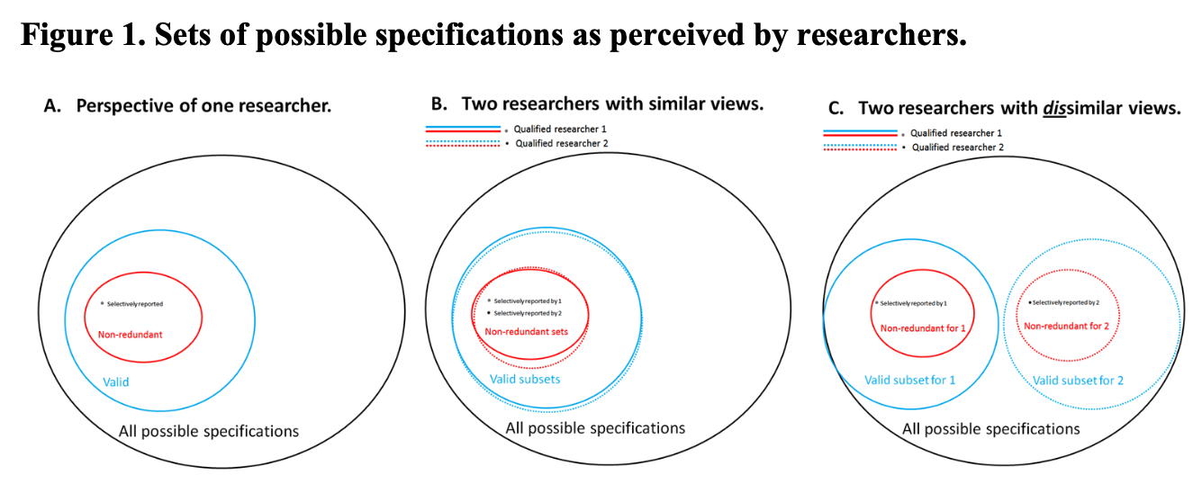
- The solution (according to Simonsohn, Simmons, & Nelson, 2015: specify all “reasonable” models and assess the distribution of effects
Figure 1 Simonsohn, Simmons, & Nelson, 2015
steps for conducting SCA
- Specify all reasonable models
- Plot specification curve showing estimates/model fits as a function of analytic decisions or model parameters
- Test how consistent the curve results are against a null hypothesis
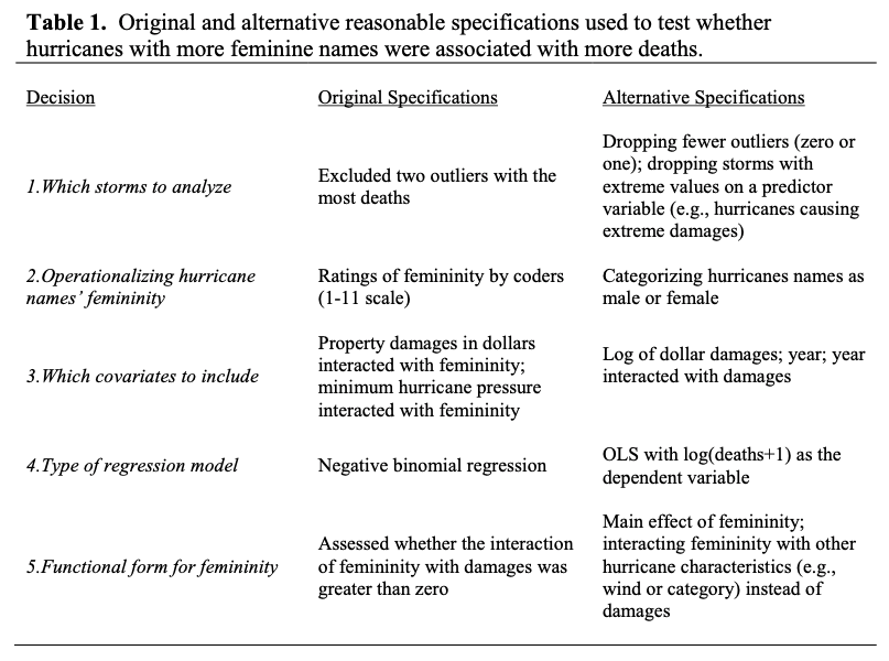
1. Reasonable specifications should be:
- Consistent with theory
- Expected to be statistically valid
- Non-redundant
Table 1 Simonsohn, Simmons, & Nelson, 2015
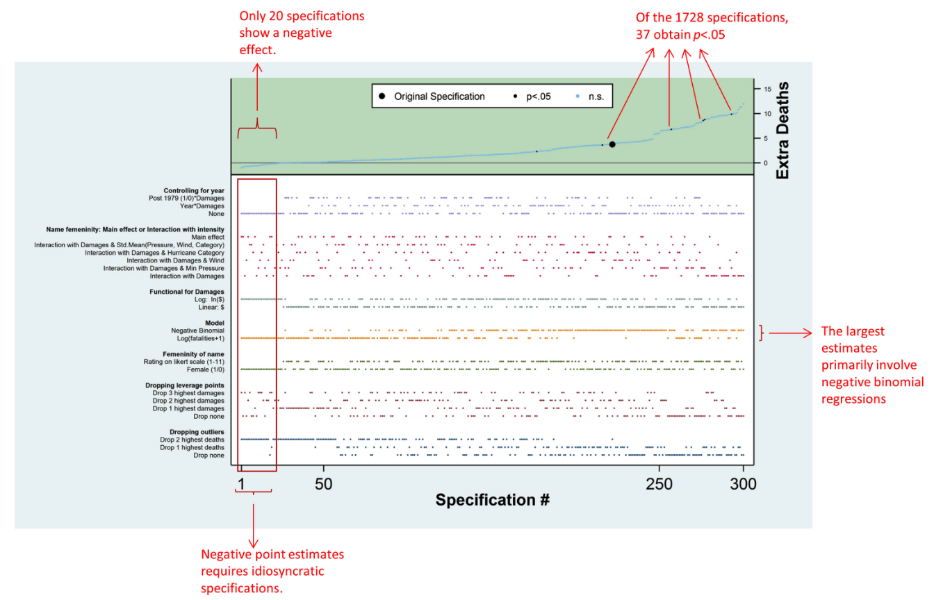
2. Descriptive specification curve
Figure 2 Simonsohn, Simmons, & Nelson, 2015
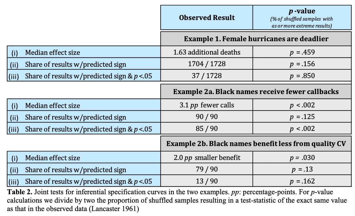
3. Inferential statistics
- Use permutation testing to run many specification curve analyses and create a null distribution
- Potential questions to test versus null:
- Is the median effect size in the observed curve statistically different than in the null distribution?
- Is the share of dominant signs (e.g., positive or negative effects) different than the null?
- Is the share of dominant signs that are statistically significant different than the null?
Table 2 Simonsohn, Simmons, & Nelson, 2015
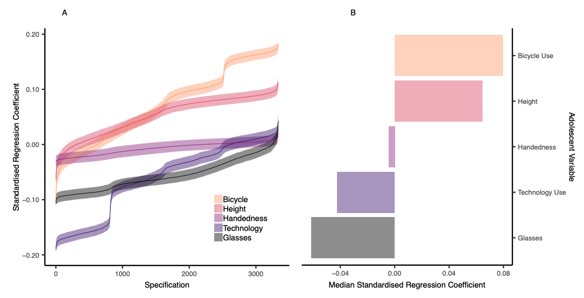
- Also possible to compare specification surves between two variables of interest
Figure 6 Orben & Przybylski, 2019
examples
programming resources
load packages
if (!require(tidyverse)) {
  install.packages('tidyverse')
}
if (!require(purrr)) {
  install.packages('purrr')
}
if (!require(broom)) {
  install.packages('broom')
}
if (!require(cowplot)) {
  install.packages('cowplot')
}
if (!require(MuMIn)) {
  install.packages('MuMIn')
}
run multiple models using map from purrr
- Note that if you are running linear mixed effects models, you can use the
broom.mixedinstead of thebroompackage to tidy the model output
# specify models
models = list(mpg ~ cyl,
              mpg ~ cyl + hp,
              mpg ~ cyl * hp)

# run models and extract parameter estimates and stats
(model_params = map(models, ~lm(.x,  data = mtcars)) %>%
  tibble() %>%
  rename("model" = ".") %>%
  mutate(tidied = purrr::map(model, broom::tidy),
         model_num = row_number()) %>%
  select(model_num, tidied) %>%
  unnest())
## # A tibble: 9 x 6
## model_num term estimate std.error statistic p.value
## <int> <chr> <dbl> <dbl> <dbl> <dbl>
## 1 1 (Intercept) 37.9 2.07 18.3 8.37e-18
## 2 1 cyl -2.88 0.322 -8.92 6.11e-10
## 3 2 (Intercept) 36.9 2.19 16.8 1.62e-16
## 4 2 cyl -2.26 0.576 -3.93 4.80e- 4
## 5 2 hp -0.0191 0.0150 -1.27 2.13e- 1
## 6 3 (Intercept) 50.8 6.51 7.79 1.72e- 8
## 7 3 cyl -4.12 0.988 -4.17 2.67e- 4
## 8 3 hp -0.171 0.0691 -2.47 1.99e- 2
## 9 3 cyl:hp 0.0197 0.00881 2.24 3.32e- 2# run models and extract model fits
(model_fits = purrr::map(models, ~lm(.x, data = mtcars)) %>%
tibble() %>%
rename("model" = ".") %>%
mutate(model_num = row_number(),
AIC = map_dbl(model, AIC),
BIC = map_dbl(model, BIC)) %>%
select(-model))## # A tibble: 3 x 3
## model_num AIC BIC
## <int> <dbl> <dbl>
## 1 1 169. 174.
## 2 2 170. 175.
## 3 3 166. 174.# join dataframes and select model fits and parameter estimates
model_params %>%
select(model_num, term, estimate) %>%
spread(term, estimate) %>%
left_join(., model_fits) %>%
arrange(AIC)## # A tibble: 3 x 7
## model_num `(Intercept)` cyl `cyl:hp` hp AIC BIC
## <int> <dbl> <dbl> <dbl> <dbl> <dbl> <dbl>
## 1 3 50.8 -4.12 0.0197 -0.171 166. 174.
## 2 1 37.9 -2.88 NA NA 169. 174.
## 3 2 36.9 -2.26 NA -0.0191 170. 175.run all nested models using dredge from MuMIn
- max number of predictors = 30
# set na.action for dredge
options(na.action = "na.fail")

# omit NAs
mtcars.na = mtcars %>%
  na.omit()

# run full model
full.model = lm(mpg ~ cyl*hp, data = mtcars.na)

# run all possible nested models
(all.models = MuMIn::dredge(full.model, rank = "AIC", extra = "BIC"))
## Global model call: lm(formula = mpg ~ cyl * hp, data = mtcars.na)
## ---
## Model selection table
## (Int) cyl hp cyl:hp BIC df logLik AIC delta weight
## 8 50.75 -4.119 -0.17070 0.01974 173.6 5 -78.143 166.3 0.00 0.706
## 2 37.88 -2.876 173.7 3 -81.653 169.3 3.02 0.156
## 4 36.91 -2.265 -0.01912 175.4 4 -80.781 169.6 3.28 0.137
## 3 30.10 -0.06823 185.6 3 -87.619 181.2 14.95 0.000
## 1 20.09 211.7 2 -102.378 208.8 42.47 0.000
## Models ranked by AIC(x)issues with factors
run factor models using dredge
- doesn’t give parameter estimates for factors directly; you need to extract them using
MuMIn::get.models()
# run full model
full.model = lm(mpg ~ cyl*as.factor(vs), data = mtcars.na)

# run all possible nested models
MuMIn::dredge(full.model, rank = "AIC", extra = "BIC") %>%
  select(AIC, BIC, everything())
## $AIC
## [1] NA 20.09062 37.88458 39.62502 36.92673 16.61667 NA NA
## [9] NA NA
##
## $BIC
## [1] <NA> <NA> <NA> + + + <NA> <NA> <NA> <NA>
## Levels: +
##
## $`(Intercept)`
## [1] NA NA -2.875790 -3.090675 -2.728218 NA NA
## [8] NA NA NA
##
## $`as.factor(vs)`
## [1] <NA> <NA> <NA> <NA> + <NA> <NA> <NA> <NA> <NA>
## Levels: +
##
## $cyl
## [1] NA 211.6870 173.7036 176.9215 179.4598 196.5443 NA NA
## [9] NA NA
##
## $`as.factor(vs):cyl`
## [1] NA 2 3 4 5 3 NA NA NA NA
##
## $df
## [1] NA -102.37776 -81.65321 -81.52927 -81.06558 -93.07356
## [7] NA NA NA NA
##
## $logLik
## [1] NA 208.7555 169.3064 171.0585 172.1312 192.1471 NA NA
## [9] NA NA
##
## $delta
## [1] NA 39.449099 0.000000 1.752124 2.824753 22.840708 NA
## [8] NA NA NA
##
## $weight
## model weights
## [1] NA NA NA NA NA NA NA NA NA NA
##
## attr(,"model.calls")
## attr(,"model.calls")$<NA>
## NULL
##
## attr(,"model.calls")$`1`
## lm(formula = mpg ~ 1, data = mtcars.na)
##
## attr(,"model.calls")$`3`
## lm(formula = mpg ~ cyl + 1, data = mtcars.na)
##
## attr(,"model.calls")$`4`
## lm(formula = mpg ~ as.factor(vs) + cyl + 1, data = mtcars.na)
##
## attr(,"model.calls")$`8`
## lm(formula = mpg ~ as.factor(vs) + cyl + as.factor(vs):cyl +
## 1, data = mtcars.na)
##
## attr(,"model.calls")$`2`
## lm(formula = mpg ~ as.factor(vs) + 1, data = mtcars.na)
##
## attr(,"model.calls")$<NA>
## NULL
##
## attr(,"model.calls")$<NA>
## NULL
##
## attr(,"model.calls")$<NA>
## NULL
##
## attr(,"model.calls")$<NA>
## NULL
##
## attr(,"global")
##
## Call:
## lm(formula = mpg ~ cyl * as.factor(vs), data = mtcars.na)
##
## Coefficients:
## (Intercept) cyl as.factor(vs)1 cyl:as.factor(vs)1
## 36.927 -2.728 5.013 -1.074run factor models using map
# specify models
models = list(mpg ~ 1,
              mpg ~ cyl,
              mpg ~ as.factor(vs),
              mpg ~ cyl + as.factor(vs),
              mpg ~ cyl*as.factor(vs))

# run models and extract parameter estimates and stats
model_params = map(models, ~lm(.x,  data = mtcars)) %>%
  tibble() %>%
  rename("model" = ".") %>%
  mutate(tidied = purrr::map(model, broom::tidy),
         model_num = row_number()) %>%
  select(model_num, tidied) %>%
  unnest()

# run models and extract model fits
model_fits = purrr::map(models, ~lm(.x,  data = mtcars)) %>%
  tibble() %>%
  rename("model" = ".") %>%
  mutate(model_num = row_number(),
         AIC = map_dbl(model, AIC),
         BIC = map_dbl(model, BIC)) %>%
  select(-model)

# join dataframes and select model fits and parameter estimates
(models.sca = model_params %>%
  select(model_num, term, estimate) %>%
  spread(term, estimate) %>%
  left_join(., model_fits) %>%
  arrange(AIC)%>%
  select(AIC, BIC, everything()))
## # A tibble: 5 x 7
## AIC BIC model_num `(Intercept)` `as.factor(vs)1` cyl `cyl:as.factor(vs)…
## <dbl> <dbl> <int> <dbl> <dbl> <dbl> <dbl>
## 1 169. 174. 2 37.9 NA -2.88 NA
## 2 171. 177. 4 39.6 -0.939 -3.09 NA
## 3 172. 179. 5 36.9 5.01 -2.73 -1.07
## 4 192. 197. 3 16.6 7.94 NA NA
## 5 209. 212. 1 20.1 NA NA NAplot specification curve
- Panel A = model fit of each model specification
- Panel B = variables included in each model specification
- Null model (intercept only) is highlighted in blue
- Models with lower AIC values than the null model are highlighted in red
# specify mpg ~ 1 as the null model for comparison
null.df = models.sca %>%
  filter(model_num == 1)

# tidy for plotting
plot.data = models.sca %>%
  arrange(AIC) %>%
  mutate(specification = row_number(),
         better.fit = ifelse(AIC == null.df$AIC, "equal",
                      ifelse(AIC < null.df$AIC, "yes","no")))

# get names of variables included in model
variable.names = names(select(plot.data, -model_num, -starts_with("better"), -specification, -AIC, -BIC))

# plot top panel
top = plot.data %>%
  ggplot(aes(specification, AIC, color = better.fit)) +
    geom_point(shape = "|", size = 4) +
    geom_hline(yintercept = null.df$AIC, linetype = "dashed", color = "lightblue") +
    scale_color_manual(values = c("lightblue", "red")) +
    labs(x = "", y = "AIC\n") +
    theme_minimal(base_size = 11) +
    theme(legend.title = element_text(size = 10),
          legend.text = element_text(size = 9),
          axis.text = element_text(color = "black"),
          axis.line = element_line(colour = "black"),
          legend.position = "none",
          panel.grid.major = element_blank(),
          panel.grid.minor = element_blank(),
          panel.border = element_blank(),
          panel.background = element_blank())

# plot bottom panel
bottom = plot.data %>%
  gather(variable, value, eval(variable.names)) %>%
  mutate(value = ifelse(!is.na(value), "|", "")) %>%
  ggplot(aes(specification, variable, color = better.fit)) +
    geom_text(aes(label = value)) +
    scale_color_manual(values = c("lightblue", "red")) +
    labs(x = "\nspecification number", y = "variables\n") +
    theme_minimal(base_size = 11) +
    theme(legend.title = element_text(size = 10),
          legend.text = element_text(size = 9),
          axis.text = element_text(color = "black"),
          axis.line = element_line(colour = "black"),
          legend.position = "none",
          panel.grid.major = element_blank(),
          panel.grid.minor = element_blank(),
          panel.border = element_blank(),
          panel.background = element_blank())

# join panels
cowplot::plot_grid(top, bottom, ncol = 1, align = "v", labels = c('A', 'B'))
reorder and rename variables
- make the plot prettier
# set plotting order for variables based on number of times it's included in better fitting models
order = plot.data %>%
  arrange(AIC) %>%
  mutate(better.fit.num = ifelse(better.fit == "yes", 1, 0)) %>%
  rename("intercept" = `(Intercept)`,
         "vs" = `as.factor(vs)1`,
         "cyl x vs" = `cyl:as.factor(vs)1`) %>%
  gather(variable, value, -model_num, -starts_with("better"), -specification, -AIC, -BIC) %>%
  filter(!is.na(value)) %>%
  group_by(variable) %>%
  mutate(order = sum(better.fit.num)) %>%
  select(variable, order) %>%
  unique()

# rename variables and plot bottom panel
bottom = plot.data %>%
  gather(variable, value, eval(variable.names)) %>%
  mutate(value = ifelse(!is.na(value), "|", ""),
         variable = ifelse(variable == "(Intercept)", "intercept",
                    ifelse(variable == "as.factor(vs)1", "vs",
                    ifelse(variable == "cyl:as.factor(vs)1", "cyl x vs", variable)))) %>%
  left_join(., order, by = "variable") %>%
  ggplot(aes(specification, reorder(variable, order), color = better.fit)) +
    geom_text(aes(label = value)) +
    scale_color_manual(values = c("lightblue", "red")) +
    labs(x = "\nspecification number", y = "variables\n") +
    theme_minimal(base_size = 11) +
    theme(legend.title = element_text(size = 10),
          legend.text = element_text(size = 9),
          axis.text = element_text(color = "black"),
          axis.line = element_line(colour = "black"),
          legend.position = "none",
          panel.grid.major = element_blank(),
          panel.grid.minor = element_blank(),
          panel.border = element_blank(),
          panel.background = element_blank())

# join panels
cowplot::plot_grid(top, bottom, ncol = 1, align = "v", labels = c('A', 'B'))
a more complicated example
run all nested models using dredge
# run full model
full.model = lm(mpg ~ cyl + disp + hp + drat + wt + qsec + as.factor(vs) + am + gear + carb, data = mtcars.na)

# run all possible nested models
models.sca = MuMIn::dredge(full.model, rank = "AIC", extra = "BIC")
plot specification curve
- compare model fits to a base model of mpg ~ 1 + cyl
# specify mpg ~ 1 as the null model for comparison
null.df = models.sca %>%
  filter(df == 3 & !is.na(cyl))

# tidy for plotting
plot.data = models.sca %>%
  arrange(AIC) %>%
  mutate(specification = row_number(),
         better.fit = ifelse(AIC == null.df$AIC, "equal",
                      ifelse(AIC < null.df$AIC, "yes","no"))) %>%
  gather(variable, value, -starts_with("better"), -specification, -AIC, -BIC, -df, -logLik, -delta, -weight) %>%
  mutate(variable = gsub("[()]", "", variable),
         variable = gsub("Intercept", "intercept", variable),
         variable = gsub("as.factor(vs)", "vs", variable)) %>%
  spread(variable, value)

# get names of variables included in model
variable.names = names(select(plot.data, -starts_with("better"), -specification, -AIC, -BIC, -df, -logLik, -delta, -weight))

# plot top panel
top = plot.data %>%
  ggplot(aes(specification, AIC, color = better.fit)) +
    geom_point(shape = "|", size = 4) +
    geom_hline(yintercept = null.df$AIC, linetype = "dashed", color = "lightblue") +
    scale_color_manual(values = c("lightblue", "black", "red")) +
    labs(x = "", y = "AIC\n") +
    theme_minimal(base_size = 11) +
    theme(legend.title = element_text(size = 10),
          legend.text = element_text(size = 9),
          axis.text = element_text(color = "black"),
          axis.line = element_line(colour = "black"),
          legend.position = "none",
          panel.grid.major = element_blank(),
          panel.grid.minor = element_blank(),
          panel.border = element_blank(),
          panel.background = element_blank())

# set plotting order for variables based on number of times it's included in better fitting models
order = plot.data %>%
  arrange(AIC) %>%
  mutate(better.fit.num = ifelse(better.fit == "yes", 1, 0)) %>%
  gather(variable, value, eval(variable.names)) %>%
  filter(!is.na(value)) %>%
  group_by(variable) %>%
  mutate(order = sum(better.fit.num)) %>%
  select(variable, order) %>%
  unique()

# rename variables and plot bottom panel
bottom = plot.data %>%
  gather(variable, value, eval(variable.names)) %>%
  mutate(value = ifelse(!is.na(value), "|", ""),
         variable = ifelse(variable == "(Intercept)", "intercept",
                    ifelse(variable == "as.factor(vs)1", "vs", variable))) %>%
  left_join(., order, by = "variable") %>%
  ggplot(aes(specification, reorder(variable, order), color = better.fit)) +
    geom_text(aes(label = value)) +
    scale_color_manual(values = c("lightblue", "black", "red")) +
    labs(x = "\nspecification number", y = "variables\n") +
    theme_minimal(base_size = 11) +
    theme(legend.title = element_text(size = 10),
          legend.text = element_text(size = 9),
          axis.text = element_text(color = "black"),
          axis.line = element_line(colour = "black"),
          legend.position = "none",
          panel.grid.major = element_blank(),
          panel.grid.minor = element_blank(),
          panel.border = element_blank(),
          panel.background = element_blank())

# join panels
cowplot::plot_grid(top, bottom, ncol = 1, align = "v", labels = c('A', 'B'))
coefficient specification curve
Rather than plotting model fit, you can also plot curves for associations of interest and determine how inclusion of other variables or analytic decisions affects the association
mpg ~ wt
Use the same method with a different association of interest ### extract coefficients and p-values
# extract parameter estimate (step-by-step output)
MuMIn::get.models(models.sca, subset = TRUE) %>%
  tibble() %>%
  rename("model" = ".")
## # A tibble: 1,024 x 1
## model
## <named list>
## 1 <lm>
## 2 <lm>
## 3 <lm>
## 4 <lm>
## 5 <lm>
## 6 <lm>
## 7 <lm>
## 8 <lm>
## 9 <lm>
## 10 <lm>
## # … with 1,014 more rowsMuMIn::get.models(models.sca, subset = TRUE) %>%
tibble() %>%
rename("model" = ".") %>%
mutate(tidied = purrr::map(model, broom::tidy),
model_num = row_number()) %>%
select(model_num, tidied) %>%
unnest()## # A tibble: 6,144 x 6
## model_num term estimate std.error statistic p.value
## <int> <chr> <dbl> <dbl> <dbl> <dbl>
## 1 1 (Intercept) 9.62 6.96 1.38 0.178
## 2 1 am 2.94 1.41 2.08 0.0467
## 3 1 qsec 1.23 0.289 4.25 0.000216
## 4 1 wt -3.92 0.711 -5.51 0.00000695
## 5 2 (Intercept) 17.4 9.32 1.87 0.0721
## 6 2 am 2.93 1.40 2.09 0.0458
## 7 2 hp -0.0176 0.0142 -1.25 0.223
## 8 2 qsec 0.811 0.439 1.85 0.0757
## 9 2 wt -3.24 0.890 -3.64 0.00114
## 10 3 (Intercept) 12.9 7.47 1.73 0.0958
## # … with 6,134 more rows# extract parameter estimate
(model_params = MuMIn::get.models(models.sca, subset = TRUE) %>%
tibble() %>%
rename("model" = ".") %>%
mutate(tidied = purrr::map(model, broom::tidy),
model_num = row_number()) %>%
select(model_num, tidied) %>%
unnest() %>%
select(model_num, term, estimate) %>%
spread(term, estimate)) %>%
select(-starts_with("sd"))## # A tibble: 1,024 x 12
## model_num `(Intercept)` am `as.factor(vs)1` carb cyl disp drat
## <int> <dbl> <dbl> <dbl> <dbl> <dbl> <dbl> <dbl>
## 1 1 9.62 2.94 NA NA NA NA NA
## 2 2 17.4 2.93 NA NA NA NA NA
## 3 3 12.9 3.51 NA -0.489 NA NA NA
## 4 4 14.4 3.47 NA NA NA 0.0112 NA
## 5 5 38.8 NA NA NA -0.942 NA NA
## 6 6 6.44 3.31 NA NA NA 0.00769 NA
## 7 7 39.6 NA NA -0.486 -1.29 NA NA
## 8 8 9.92 2.96 NA -0.602 NA NA 1.21
## 9 9 17.7 3.32 NA -0.336 NA NA NA
## 10 10 14.9 2.47 NA NA -0.354 NA NA
## # … with 1,014 more rows, and 4 more variables: gear <dbl>, hp <dbl>,
## # qsec <dbl>, wt <dbl># extract p-values for the intercept term
(model_ps = MuMIn::get.models(models.sca, subset = TRUE) %>%
tibble() %>%
rename("model" = ".") %>%
mutate(tidied = purrr::map(model, broom::tidy),
model_num = row_number()) %>%
select(model_num, tidied) %>%
unnest() %>%
filter(term == "wt") %>%
ungroup() %>%
select(model_num, estimate, std.error, p.value))## # A tibble: 512 x 4
## model_num estimate std.error p.value
## <int> <dbl> <dbl> <dbl>
## 1 1 -3.92 0.711 0.00000695
## 2 2 -3.24 0.890 0.00114
## 3 3 -3.43 0.820 0.000269
## 4 4 -4.08 1.19 0.00208
## 5 5 -3.17 0.741 0.000199
## 6 6 -4.59 1.17 0.000529
## 7 7 -3.16 0.742 0.000211
## 8 8 -3.11 0.905 0.00199
## 9 9 -3.08 0.925 0.00263
## 10 10 -3.64 0.910 0.000436
## # … with 502 more rowsplot specification curve
- red = statistically significant values at p < .05
- black = p > .05
# merge and tidy for plotting
plot.data = left_join(model_ps, model_params, by = "model_num") %>%
  arrange(estimate) %>%
  mutate(specification = row_number(),
         significant.p = ifelse(p.value < .05, "yes", "no")) %>%
  gather(variable, value, -estimate, -specification, -model_num, -std.error, -p.value, -significant.p) %>%
  mutate(variable = gsub("[()]", "", variable),
         variable = gsub("Intercept", "intercept", variable),
         variable = gsub("as.factor(vs)1", "vs", variable)) %>%
  spread(variable, value)

# get names of variables included in model
variable.names = names(select(plot.data, -estimate, -specification, -model_num, -std.error, -p.value, -significant.p))

# plot top panel
top = plot.data %>%
  ggplot(aes(specification, estimate, color = significant.p)) +
    geom_point(shape = "|", size = 4) +
    #geom_hline(yintercept = null.df$AIC, linetype = "dashed", color = "lightblue") +
    scale_color_manual(values = c("black", "red")) +
    labs(x = "", y = "regression coefficient\n") +
    theme_minimal(base_size = 11) +
    theme(legend.title = element_text(size = 10),
          legend.text = element_text(size = 9),
          axis.text = element_text(color = "black"),
          axis.line = element_line(colour = "black"),
          legend.position = "none",
          panel.grid.major = element_blank(),
          panel.grid.minor = element_blank(),
          panel.border = element_blank(),
          panel.background = element_blank())

# set plotting order for variables based on number of times it's included in better fitting models
order = plot.data %>%
  arrange(estimate) %>%
  mutate(significant.p.num = ifelse(significant.p == "yes", 1, 0)) %>%
  gather(variable, value, eval(variable.names)) %>%
  filter(!is.na(value)) %>%
  group_by(variable) %>%
  mutate(order = sum(significant.p.num)) %>%
  select(variable, order) %>%
  unique()

# rename variables and plot bottom panel
bottom = plot.data %>%
  gather(variable, value, eval(variable.names)) %>%
  mutate(value = ifelse(!is.na(value), "|", ""),
         variable = ifelse(variable == "(Intercept)", "intercept",
                    ifelse(variable == "as.factor(vs)1", "vs", variable))) %>%
  left_join(., order, by = "variable") %>%
  ggplot(aes(specification, reorder(variable, order), color = significant.p)) +
    geom_text(aes(label = value)) +
    scale_color_manual(values = c("black", "red")) +
    labs(x = "\nspecification number", y = "variables\n") +
    theme_minimal(base_size = 11) +
    theme(legend.title = element_text(size = 10),
          legend.text = element_text(size = 9),
          axis.text = element_text(color = "black"),
          axis.line = element_line(colour = "black"),
          legend.position = "none",
          panel.grid.major = element_blank(),
          panel.grid.minor = element_blank(),
          panel.border = element_blank(),
          panel.background = element_blank())

# join panels
(wt = cowplot::plot_grid(top, bottom, ncol = 1, align = "v", labels = c('A', 'B')))
mpg ~ cyl
extract coefficients
# extract p-values for the intercept term
model_ps = MuMIn::get.models(models.sca, subset = TRUE) %>%
  tibble() %>%
  rename("model" = ".") %>%
  mutate(tidied = purrr::map(model, broom::tidy),
         model_num = row_number()) %>%
  select(model_num, tidied) %>%
  unnest() %>%
  filter(term == "cyl") %>%
  ungroup() %>%
  select(model_num, estimate, std.error, p.value)
plot specification curve
# merge and tidy for plotting
plot.data = left_join(model_ps, model_params, by = "model_num") %>%
  arrange(estimate) %>%
  mutate(specification = row_number(),
         significant.p = ifelse(p.value < .05, "yes", "no")) %>%
  gather(variable, value, -estimate, -specification, -model_num, -std.error, -p.value, -significant.p) %>%
  mutate(variable = gsub("[()]", "", variable),
         variable = gsub("Intercept", "intercept", variable),
         variable = gsub("as.factor(vs)1", "vs", variable)) %>%
  spread(variable, value)

# get names of variables included in model
variable.names = names(select(plot.data, -estimate, -specification, -model_num, -std.error, -p.value, -significant.p))

# plot top panel
top = plot.data %>%
  ggplot(aes(specification, estimate, color = significant.p)) +
    geom_point(shape = "|", size = 4) +
    #geom_hline(yintercept = null.df$AIC, linetype = "dashed", color = "lightblue") +
    scale_color_manual(values = c("black", "red")) +
    labs(x = "", y = "regression coefficient\n") +
    theme_minimal(base_size = 11) +
    theme(legend.title = element_text(size = 10),
          legend.text = element_text(size = 9),
          axis.text = element_text(color = "black"),
          axis.line = element_line(colour = "black"),
          legend.position = "none",
          panel.grid.major = element_blank(),
          panel.grid.minor = element_blank(),
          panel.border = element_blank(),
          panel.background = element_blank())

# set plotting order for variables based on number of times it's included in better fitting models
order = plot.data %>%
  arrange(estimate) %>%
  mutate(significant.p.num = ifelse(significant.p == "yes", 1, 0)) %>%
  gather(variable, value, eval(variable.names)) %>%
  filter(!is.na(value)) %>%
  group_by(variable) %>%
  mutate(order = sum(significant.p.num)) %>%
  select(variable, order) %>%
  unique()

# rename variables and plot bottom panel
bottom = plot.data %>%
  gather(variable, value, eval(variable.names)) %>%
  mutate(value = ifelse(!is.na(value), "|", ""),
         variable = ifelse(variable == "(Intercept)", "intercept",
                    ifelse(variable == "as.factor(vs)1", "vs", variable))) %>%
  left_join(., order, by = "variable") %>%
  ggplot(aes(specification, reorder(variable, order), color = significant.p)) +
    geom_text(aes(label = value)) +
    scale_color_manual(values = c("black", "red")) +
    labs(x = "\nspecification number", y = "variables\n") +
    theme_minimal(base_size = 11) +
    theme(legend.title = element_text(size = 10),
          legend.text = element_text(size = 9),
          axis.text = element_text(color = "black"),
          axis.line = element_line(colour = "black"),
          legend.position = "none",
          panel.grid.major = element_blank(),
          panel.grid.minor = element_blank(),
          panel.border = element_blank(),
          panel.background = element_blank())

# join panels
(cyl = cowplot::plot_grid(top, bottom, ncol = 1, align = "v", labels = c('A', 'B')))
add confidence intervals
extract CIs
# calculate 95% CIs and extract p-values for the wt term
(model_ps = MuMIn::get.models(models.sca, subset = TRUE) %>%
  tibble() %>%
  rename("model" = ".") %>%
  mutate(tidied = purrr::map(model, broom::tidy, conf.int = TRUE),
         model_num = row_number()) %>%
  select(model_num, tidied) %>%
  unnest() %>%
  filter(term == "wt") %>%
  ungroup() %>%
  select(model_num, estimate, std.error, p.value, conf.low, conf.high))
## # A tibble: 512 x 6
## model_num estimate std.error p.value conf.low conf.high
## <int> <dbl> <dbl> <dbl> <dbl> <dbl>
## 1 1 -3.92 0.711 0.00000695 -5.37 -2.46
## 2 2 -3.24 0.890 0.00114 -5.06 -1.41
## 3 3 -3.43 0.820 0.000269 -5.12 -1.75
## 4 4 -4.08 1.19 0.00208 -6.54 -1.63
## 5 5 -3.17 0.741 0.000199 -4.68 -1.65
## 6 6 -4.59 1.17 0.000529 -6.98 -2.19
## 7 7 -3.16 0.742 0.000211 -4.68 -1.64
## 8 8 -3.11 0.905 0.00199 -4.97 -1.25
## 9 9 -3.08 0.925 0.00263 -4.98 -1.17
## 10 10 -3.64 0.910 0.000436 -5.51 -1.78
## # … with 502 more rowsplot
# merge and tidy for plotting
plot.data = left_join(model_ps, model_params, by = "model_num") %>%
  arrange(estimate) %>%
  mutate(specification = row_number(),
         significant.p = ifelse(p.value < .05, "yes", "no")) %>%
  gather(variable, value, -estimate, -specification, -model_num, -std.error, -p.value, -significant.p, -contains("conf")) %>%
  mutate(variable = gsub("[()]", "", variable),
         variable = gsub("Intercept", "intercept", variable),
         variable = gsub("as.factor(vs)1", "vs", variable)) %>%
  spread(variable, value)

# get names of variables included in model
variable.names = names(select(plot.data, -estimate, -specification, -model_num, -std.error, -p.value, -significant.p, -contains("conf")))

# plot top panel
top = plot.data %>%
  ggplot(aes(specification, estimate, color = significant.p)) +
    geom_pointrange(aes(ymin = conf.low, ymax = conf.high), size = .25, shape = "", alpha = .5) +
    geom_point(size = .25) +
    scale_color_manual(values = c("black", "red")) +
    labs(x = "", y = "regression coefficient\n") +
    theme_minimal(base_size = 11) +
    theme(legend.title = element_text(size = 10),
          legend.text = element_text(size = 9),
          axis.text = element_text(color = "black"),
          axis.line = element_line(colour = "black"),
          legend.position = "none",
          panel.grid.major = element_blank(),
          panel.grid.minor = element_blank(),
          panel.border = element_blank(),
          panel.background = element_blank())

# set plotting order for variables based on number of times it's included in better fitting models
order = plot.data %>%
  arrange(estimate) %>%
  mutate(significant.p.num = ifelse(significant.p == "yes", 1, 0)) %>%
  gather(variable, value, eval(variable.names)) %>%
  filter(!is.na(value)) %>%
  group_by(variable) %>%
  mutate(order = sum(significant.p.num)) %>%
  select(variable, order) %>%
  unique()

# rename variables and plot bottom panel
bottom = plot.data %>%
  gather(variable, value, eval(variable.names)) %>%
  mutate(value = ifelse(!is.na(value), "|", ""),
         variable = ifelse(variable == "(Intercept)", "intercept",
                    ifelse(variable == "as.factor(vs)1", "vs", variable))) %>%
  left_join(., order, by = "variable") %>%
  ggplot(aes(specification, reorder(variable, order), color = significant.p)) +
    geom_text(aes(label = value)) +
    scale_color_manual(values = c("black", "red")) +
    labs(x = "\nspecification number", y = "variables\n") +
    theme_minimal(base_size = 11) +
    theme(legend.title = element_text(size = 10),
          legend.text = element_text(size = 9),
          axis.text = element_text(color = "black"),
          axis.line = element_line(colour = "black"),
          legend.position = "none",
          panel.grid.major = element_blank(),
          panel.grid.minor = element_blank(),
          panel.border = element_blank(),
          panel.background = element_blank())

# join panels
(wt_ci = cowplot::plot_grid(top, bottom, ncol = 1, align = "v", labels = c('A', 'B')))
next steps
… Inferential statistics using specification curves!